
DBMS Interview Notes
Data & DBMS basics, Architecture, ER & Relational Model, SQL (DDL, DQL, DML, DCL, TCL), Transactions & Concurrency, Normalization, Indexing, Replication, Partitioning and Sharding
Table of Contents
Introduction to DBMS
What is Data?
- Data is a collection of raw, unorganized facts such as:
- Text, numbers, observations, symbols, descriptions, etc.
- It has no meaning on its own unless processed.
- Measured in:
- Bits and Bytes (basic storage units)
- Data can be recorded, but it becomes meaningful only after processing.
Types of Data
a. Quantitative Data
- Numerical in nature
- Examples:
- Weight
- Volume
- Cost
b. Qualitative Data
- Descriptive (non-numerical)
- Examples:
- Name
- Gender
- Hair color
What is Information?
- Information is processed, organized, and structured data.
- It:
- Provides context
- Helps in decision-making
- Makes data meaningful
Example:
- Raw Data: List of people in a locality
- Information (after processing):
- 100 senior citizens
- Sex ratio = 1.1
- 100 newborn babies
Data vs Information
| Data | Information |
|---|---|
| Raw and unorganized | Processed and organized |
| No meaning alone | Meaningful |
| Independent | Depends on data |
| Individual facts | Big-picture understanding |
| Represented as numbers, graphs, figures | Presented as words, ideas |
| Not useful for decisions | Useful for decision-making |
What is a Database?
- A database is an electronic system where:
- Data is stored
- Easily accessed, managed, and updated
- To efficiently use data, we need a DBMS.
What is DBMS?
- DBMS (Database Management System):
- A system that manages databases
- Consists of:
- Data + Software to handle it
Functions of DBMS:
- Store data
- Retrieve data
- Update data
- Delete data
Goal:
- Provide efficient and convenient data access
e.g., MySQL, PostgreSQL, Oracle
DBMS vs File System
Problems in File System:
- Data redundancy (duplicate data)
- Data inconsistency
- Difficulty in accessing data
- Data isolation
- Integrity problems
- Atomicity problems
- Concurrent access issues
- Security problems
Why DBMS? (Advantages)
- Eliminates redundancy
- Ensures consistency
- Easy data access
- Better security
- Supports concurrency
- Maintains integrity
- Provides atomic operations
What is an RDBMS?
Relational DBMS is based on the relational model introduced by E.F. Codd. Data is structured into tables (relations) consisting of rows (tuples/records) and columns (attributes/fields). Relationships are established using Foreign Keys.
What is SQL?
Structured Query Language is the standardized domain-specific language used to store, manipulate, and retrieve data from an RDBMS. Note: SQL is a query language, NOT a database engine.
SQL vs MySQL
SQL is the standardized language definition, whereas MySQL is an open-source Relational Database Management System that uses SQL as its primary query interface.
SQL queries are logically processed in a specific sequence distinct from their written order: 1. FROM & JOIN (Identify tables & merge) → 2. ON (Join conditions) → 3. WHERE (Filter raw rows) → 4. GROUP BY (Aggregate rows) → 5. HAVING (Filter groups) → 6. SELECT (Choose columns) → 7. DISTINCT (Remove duplicates) → 8. ORDER BY (Sort result) → 9. LIMIT / OFFSET (Paginate)
DBMS Architecture
View of Data (Three-Schema Architecture)
Purpose
- DBMS provides an abstract view of data.
- Hides details of how data is stored and maintained.
- Enables multiple users to access same data with different views.
- Physical Level(Internal Level): Describes how data is stored physically
- This is the lowest level of abstraction and describes how the data is actually stored in the database, including data structures, file storage, and indexing methods.
- It deals with the physical storage of data and focuses on optimizing storage and retrieval.
- Physical Level is managed by database administrator.
- Logical Level(Conceptual Level): Describes what data is stored and relationships
- This middle level of abstraction defines what data is stored in the database and the relationships among those data. It involves the structure of the entire database.
- It hides the details of the physical storage and focuses on the logical relationships between different data entities.
- View Level(External Level): Provides different views to different users
- This is the highest level of abstraction and describes only a part of the entire database. It shows the data that is relevant to a specific group of users or application, such as views or user interfaces.
- It provides different views of the database to different users, allowing them to access the data without worrying about its complexity.

Instances and Schemas
a. Instance
- Data in DB at a particular moment
- Changes frequently
b. Schema
- Structure/design of database
- Changes rarely
Types of Schemas
- Physical Schema
- Logical Schema
- View Schemas (Subschemas)
Data independence: -Data independence is defined as the capacity to change the schema at one level of a database system without having to change the schema at the next higher level.
Types of data independence :
- 1. Physical data independence: Physical data independence is the ability to modify internal schema without changing the conceptual schema.
- Modification at the physical level is occasionally necessary in order to improve performance. It refers to the immunity of the conceptual schema to change in the internal schema.
- Examples of physical data independence are reorganizations of files, adding a new access path or modifying indexes, etc.
- 2. Logical data independence: Logical data independence is the ability to modify the conceptual schema without having to change the external schemas or application programs. It refers to the immunity of the external model to changes in the conceptual model. Examples of logical data independence are addition/removal of entities.
Data Models
- Define how data is structured at logical level
Examples:
- ER Model
- Relational Model
- Object-Oriented Model
- Object-Relational Model
Database Administrator (DBA)
Definition
- Person with central control over DB and programs
Functions of DBA
- Schema definition
- Storage structure & access methods
- Schema modifications
- Authorization control
- Routine maintenance:
- Backup
- Security patches
- Upgrades
DBMS Application Architectures
a. 1-Tier Architecture
- Client + Server + DB on same machine
b. 2-Tier Architecture
- Application divided into 2 parts
Components:
- Client → sends queries
- Server → processes DB requests
c. 3-Tier Architecture
- Application divided into 3 layers
Layers:
- Client (Frontend)
- Application Server (Business Logic)
- Database Server
Features:
- Client does
NOTdirectly access DB - App server handles logic
Advantages:
- Scalability
- Better Security
- Data Integrity

ER Model: Entities & Attributes
Introduction of ER Model
The Entity-Relationship (ER) Model is a conceptual framework used to describe the structure of a database in terms of entities, relationships, and attributes.
It is commonly used in the design phase of database development to visually represent the data and its relationships before implementation.
Why Use ER Diagrams In DBMS?
- ER diagrams represent the E-R model in a database, making them easy to convert into relations (tables).
- ER diagrams require no technical knowledge and no hardware support.
- These diagrams are very easy to understand and easy to create even for a new user.
- It gives a standard solution for visualizing the data logically.
Components of ER Diagram

Entity
An entity is a thing in a real-world with independent existence.
An entity is a thing or an object in the real world that is distinguishable from other object based on the values of the attributes it possesses.
An entity can be of two types :
- Tangible Entity : Entities that exist in the real world physically. Example: Person, car, etc.
- Intangible Entity : Entities that exist only logically and have no physical existence. Example: Bank Account, etc.
Entity Type : It refers to the category that a particular entity belongs to.
Entity Set?
An entity set is a collection or set of all entities of a particular entity type at any point in time. The type of all the entities should be the same.

For Example, E1 is an entity having Entity Type Student and the set of all students is called Entity Set.
In ER diagram, Entity Type is represented as:
We can represent the entity set in ER Diagram but can’t represent entity in ER Diagram because entity is row and column in the relation and ER Diagram is graphical representation of data.
In ER diagram we cannot represent an entity, as entity is an instant not schema, and ER diagram is designed to understand schema.
In a relational model entity is represented by a row or a tuple or a record in a table.

| Entity | Entity Type | Entity Set |
|---|---|---|
| A thing in the real world with independent existence | A category of a particular entity | Set of all entities of a particular entity type. |
| Any particular row (a record) in a relation(table) is known as an entity. | The name of a relation (table) in RDBMS is an entity type | All rows of a relation (table) in RDBMS is entity se |
Types of Entity
There are two types of entity:
1. Strong Entity
A Strong Entity is a type of entity that has a key Attribute. Strong Entity does not depend on other Entity in the Schema. It has a primary key, that helps in identifying it uniquely, and it is represented by a rectangle. These are called Strong Entity Types.
The relationship of two strong entities is represented by a single diamond.
2. Weak Entity
Those entity type for which key attributes can’t be defined. These are called Weak Entity Types. A weak entity type is represented by a Double Rectangle.

The relationship between the weak entity type and its identifying strong entity type is called identifying relationship and it is represented by a double diamond.
Difference between Strong and Weak Entity
| Strong Entity | Weak Entity |
|---|---|
| Strong entity always has a primary key. | While a weak entity has a partial discriminator key. |
| Strong entity is not dependent on any other entity. | Weak entity depends on strong entity. |
| Strong entity is represented by a single rectangle. | Weak entity is represented by a double rectangle. |
| Two strong entity’s relationship is represented by a single diamond. | While the relation between one strong and one weak entity is represented by a double diamond. |
| Strong entities have either total participation or partial participation. | A weak entity has a total participation constraint. |
Attributes
Attributes are the properties that define the entity type.
For example, Roll_No, Name, DOB, Age, Address, and Mobile_No are the attributes that define entity type Student. In ER diagram, the attribute is represented by an oval.
While in a relational model they are represented by independent column.
Types of Attributes
- Simple Attributes- Attributes which cannot be divided further into sub parts. E.g. Age
- Key Attribute- The attribute which uniquely identifies each entity in the entity set is called the key attribute. For example,
Roll_Nowill be unique for each student. In ER diagram, the key attribute is represented by an oval with underlying lines. - Composite Attribute- Attributes which can be further divided into sub parts, as simple attributes. A composite attribute is represented by an ellipse connected to an ellipse and in a relational model by a separate column.
- Derived Attributes - The value of these types of attributes can be derived from values of other Attributes. E.g. -Age attribute can be derived from
date_of_birthand Date attribute. - Multivalued Attributes- Attributes which can have more than one value for an entity at same time. E.g. -Phone no, email, address, hobbies. A multivalued attribute is represented by a double ellipse in an ER diagram and by an independent table in a relational model.

Symbols Used in ER Model
- Rectangles: Rectangles represent Entities in the ER Model.
- Ellipses: Ellipses represent Attributes in the ER Model.
- Diamond: Diamonds represent Relationships among Entities.
- Lines: Lines represent attributes to entities and entity sets with other relationship types.
- Double Ellipse: Double Ellipses represent Multi-Valued Attributes.
- Double Rectangle: Double Rectangle represents a Weak Entity.
ER Model: Relationships & Extended ER
Relationship Type and Relationship Set
A Relationship Type represents the association between entity types. For example, ‘Enrolled in’ is a relationship type that exists between entity type Student and Course. In ER diagram, the relationship type is represented by a diamond and connecting the entities with lines.,
while in relational model sometimes through foreign key and other time by a separate table.
A set of relationships of the same type is known as a relationship set.

In an Entity-Relationship (ER) diagram, relationships between entities are represented as types, not as individual instances or data.
- Entity Types: Represent a category or class of entities (e.g., "Student," "Course").
- Relationship Types: Represent associations between entity types (e.g., "Enrolled In," which links "Student" and "Course").
- Every relationship type has three components: -
- Name
- Degree
- Structural constraints (cardinalities ratios, participation)
Name: - Every relation must have unique name.
Degree of a Relationship Set
The number of different entity sets participating in a relationship set is called the degree of a relationship set.
1. Unary Relationship: When there is only ONE entity set participating in a relation, the relationship is called a unary relationship. For example, one person is married to only one person.


2. Binary Relationship: When there are TWO entities set participating in a relationship, the relationship is called a binary relationship. For example, a Student is enrolled in a Course.
3. Ternary Relationship: When there are three entity sets participating in a relationship, the relationship is called a ternary relationship.
E.g. The University might need to record which teachers taught which subjects in which courses.

4. N-ary Relationship: When there are n entities set participating in a relationship, the relationship is called an n-ary relationship.
Structural constraints (Cardinalities Ratios, Participation)
Structural constraints in an Entity-Relationship (ER) diagram refer to the rules that govern the relationships between entities. These constraints define how many instances of an entity can or must participate in a relationship.
- Cardinality Ratios of relationships
The entities are denoted by rectangle and relationships by diamond.

There are numbers (represented by M and N) written above the lines which connect relationships and entities. These are called cardinality ratios.
These represent the maximum number of entities that can be associated with each other through relationship, R.
Types of Cardinality: There can be 4 types of cardinality –

- One-to-one (1:1) – When one entity in each entity set takes part at most once in the relationship, the cardinality is one-to-one.

E.g.-The directed line from relationship set advisor to both entities set indicates that ‘an instructor may advise at most one student, and a student may have at most one advisor’.
- One-to-many (1: N) – If entities in the first entity set take part in the relationship set at most once and entities in the second entity set take part many times (at least twice), the cardinality is said to be one-to-many.

E.g.-This indicates that an instructor may advise many students, but a student may have at most one advisor.
- Many-to-one (N:1) – If entities in the first entity set take part in the relationship set many times (at least twice), while entities in the second entity set take part at most once, the cardinality is said to be many-to-one.

E.g.-This indicates that student may have many instructors but an instructor can advise at most one student.
- Many-to-many (N: N) – The cardinality is said to be many to many if entities in both the entity sets take part many times (at least twice) in the relationship set.

E.g.-This indicates a student may have many advisors and an instructor may advise many students.
Mapping Cardinality (Cardinality Ratio)
| Type | Meaning | Example |
|---|---|---|
| One-to-One (1:1) | One ↔ One | Citizen ↔ Aadhar |
| One-to-Many (1:N) | One → Many | Citizen → Vehicles |
| Many-to-One (N:1) | Many → One | Students → Professor |
| Many-to-Many (M:N) | Many ↔ Many | Students ↔ Courses |
- Participation Constraints: Participation Constraints tell us that the participation in a relationship can either be total or partial.

When each entity in an entity set participates in a relation, it is called Total Participation. However, when all entities in the given entity set do not participate in a relation, it is called Partial Participation.
Extended ER Features
When database complexity increases, Extended ER (EER) features are used.
Generalisation (Bottom-Up Approach)
Definition
- Process of combining multiple lower-level entities into a higher-level entity based on common features.
Key Points
- Reverse of Specialisation
- Follows Bottom-Up approach
- Uses “is-a” relationship
Example
- Car, Jeep, Bus → Vehicle
- Vehicle = Superclass
- Others = Subclasses
Why Generalisation?
- Reduces data redundancy
- Makes DB simpler and more organized
Specialisation (Top-Down Approach)
Definition
- Process of dividing a higher-level entity (superclass) into lower-level entities (subclasses).
- Based on differences in features, roles, or attributes.
Key Points
- Follows Top-Down approach
- Relationship: “is-a” relationship
- Represented using a triangle in ER diagram
Example
- Person → Customer, Student, Employee
- Person = Superclass
- Others = Subclasses
Why Specialisation?
- Some attributes apply only to specific entities
- Helps represent distinct features clearly
- Improves DB design accuracy and clarity
Aggregation
Key Idea
- Relationship → converted into an entity → participates in another relationship
Aggregation is an abstraction through which we can represent relationships as higher-level entity sets.
For Example, an Employee working on a project may require some machinery. So, REQUIRE relationship is needed between the relationship WORKS_FOR and entity MACHINERY. Using aggregation, WORKS_FOR relationship with its entities EMPLOYEE and PROJECT is aggregated into a single entity and relationship REQUIRE is created between the aggregated entity and MACHINERY.

Relational Model
Relational Model (RM)
The Relational Model (RM) organizes data into relations (tables).
A relational database is a collection of tables, each with a unique name.
Basic Terminology
Table (Relation)
- A table represents a collection of related data.
Tuple (Row)
- A single row in a table
- Represents a unique record/data point
Attribute (Column)
- Columns define the properties of the relation
- Each attribute has a domain (allowed values)
Relation Schema
- Defines the structure/design of a table
- Includes:
- Relation name
- Attributes (columns)
👉 Example:
Student(ID, Name, Age)
Degree & Cardinality
- Degree → Number of attributes (columns)
- Cardinality → Number of tuples (rows)
Your notes are mostly correct. However, a few points need clarification for DBMS exams and interviews, especially Primary Key, Composite Key vs. Compound Key, Foreign Key, and Integrity Constraints. Here is the corrected and expanded version.
Relational Keys
6.1 Super Key (SK)
A Super Key is any set of one or more attributes that uniquely identifies each tuple (row) in a table.
- It may contain extra or redundant attributes.
- Every candidate key is a super key, but every super key is not a candidate key.
Example
Consider an STUDENT table
| Student_ID | Name | |
|---|---|---|
| 101 | a@gmail.com | Aman |
| 102 | b@gmail.com | Ravi |
Assume Student_ID and Email are both unique.
Examples of super keys
- {
Student_ID} - {Email}
- {
Student_ID, Name} - {
Student_ID, Email}
The last two are super keys because they uniquely identify students, even though they contain unnecessary attributes.
6.2 Candidate Key (CK)
A Candidate Key is a minimal super key that uniquely identifies each tuple.
Properties
- Uniquely identifies each row.
- Contains no redundant attributes.
- Must not contain
NULLvalues when used as a candidate key under the relational model.
Example
- {
Student_ID} - {Email}
Both are candidate keys if each value is unique and non-NULL.
{Student_ID, Name} is not a candidate key because Student_ID alone is sufficient to identify the row.
6.3 Primary Key (PK)
A Primary Key is the candidate key selected to uniquely identify each row in a table.
Properties
- Must be unique.
- Cannot contain
NULLvalues. - Only one primary key constraint can be defined per table, although it may consist of multiple columns.
- It is selected from the candidate keys; it does not necessarily have the fewest attributes among all possible keys.
Example
CREATE TABLE Student (
    Student_ID INT PRIMARY KEY,
    Email VARCHAR(100) UNIQUE,
    Name VARCHAR(50)
);
Here, Student_ID is the primary key, and Email is an alternate key if it is also a candidate key.
6.4 Alternate Key (AK)
An Alternate Key is a candidate key that is not selected as the primary key.
Example
If Student_ID and Email are candidate keys and Student_ID is selected as the primary key, then Email is an alternate key.
6.5 Foreign Key (FK)
A Foreign Key is an attribute or combination of attributes in one table that references a candidate key—usually the primary key—of the same or another table.
- Referencing table → Child table
- Referenced table → Parent table
- A foreign key may contain
NULLvalues unless restricted byNOT NULL. - Non-NULL foreign-key values must satisfy the referenced-key constraint.
Example
CREATE TABLE Department (
    Dept_ID INT PRIMARY KEY,
    Dept_Name VARCHAR(50)
);

CREATE TABLE Student (
    Student_ID INT PRIMARY KEY,
    Name VARCHAR(50),
    Dept_ID INT,
    FOREIGN KEY (Dept_ID) REFERENCES Department(Dept_ID)
);
Here, Department is the parent table, and Student is the child table.
6.6 Composite Key
A Composite Key is a key consisting of two or more attributes that together identify a row uniquely.
Example
CREATE TABLE Enrollment (
    Student_ID INT,
    Course_ID INT,
    Grade CHAR(2),
    PRIMARY KEY (Student_ID, Course_ID)
);
The combination of Student_ID and Course_ID uniquely identifies each enrollment.
6.7 Compound Key
In common DBMS teaching terminology, a Compound Key is a key composed of two or more foreign keys.
Example
An Enrollment table may contain
Student_ID→ Foreign key referencing StudentCourse_ID→ Foreign key referencing Course
Together, these columns form the primary key.
Terminology varies. In many database references, composite key and compound key are used interchangeably. The distinction above is a convention used in some courses, not a universal rule.
6.8 Surrogate Key
A Surrogate Key is an artificially generated identifier with no direct business meaning.
Properties
- Often generated automatically.
- Usually remains independent of business attributes.
- Commonly implemented using an auto-increment integer or UUID.
Example
CREATE TABLE Student (
    Student_ID INT GENERATED ALWAYS AS IDENTITY PRIMARY KEY,
    Name VARCHAR(50)
);
The exact identity-column syntax depends on the DBMS.
Relation Properties & Integrity Constraints
7. Properties of a Relation (Table)
In the relational model
- Each relation has a unique name within its schema.
- Each attribute has a unique name within the relation.
- Each cell contains a single value from its attribute's domain.
- Duplicate tuples are not allowed in a mathematical relation.
- The order of rows does not matter.
- The order of columns does not matter.
- Each attribute has a defined domain.
- The relation must satisfy applicable integrity constraints.
SQL tables can contain duplicate rows unless prevented by a key or another constraint. SQL also supports NULL values, so practical SQL tables do not always follow every property of the pure relational model.
8. Integrity Constraints
8.1 Purpose
Integrity constraints are rules that maintain the accuracy, validity, and consistency of data.
They prevent invalid data from being inserted or updated and help preserve relationships between tables.
8.2 Domain Constraints
Domain constraints restrict the values that an attribute can contain.
They may specify
- Data type
- Permitted range
- Format or set of allowed values
- Whether
NULLis permitted
Example
CREATE TABLE Student (
    Age INT CHECK (Age BETWEEN 16 AND 100)
);
This restricts Age to values between 16 and 100 when the constraint is evaluated.
Another example
Birth_Year INT CHECK (Birth_Year < 2002)This enforces the specified birth-year condition, although the condition itself depends on the application's requirements.
8.3 Entity Integrity Constraint
Entity integrity ensures that each row can be uniquely identified.
Rules
- A relation's primary key must be unique.
- Primary-key attributes cannot contain
NULLvalues.
Example
CREATE TABLE Student (
    Student_ID INT PRIMARY KEY,
    Name VARCHAR(50)
);
The database rejects duplicate or NULL Student_ID values.
8.4 Referential Integrity Constraint
Referential integrity ensures consistency between related tables.
Rules
- A non-NULL foreign-key value must match a valid referenced key.
- A foreign key may be
NULLif the column permitsNULL. - The database can define actions for deleting or updating referenced rows, such as CASCADE, SET
NULL, RESTRICT, or NO ACTION, depending on the DBMS.
Example
CREATE TABLE Department (
    Dept_ID INT PRIMARY KEY
);

CREATE TABLE Student (
    Student_ID INT PRIMARY KEY,
    Dept_ID INT,
    FOREIGN KEY (Dept_ID) REFERENCES Department(Dept_ID)
);
A student cannot reference a non-existent department. However, Dept_ID may be NULL because it has not been declared NOT NULL.
8.5 Key Constraints
Key constraints ensure that attributes designated as keys uniquely identify rows.
For example
CREATE TABLE Student (
    Student_ID INT PRIMARY KEY,
    Email VARCHAR(100) UNIQUE
);
Here, Student_ID must be unique and non-NULL. Email must satisfy the DBMS's UNIQUE constraint rules.
SQL Data Types
Common SQL Data Types
| Data Type | Description | Storage / Range | Example |
|---|---|---|---|
CHAR(n) | Fixed-length character string. | Up to 255 characters in MySQL; shorter values are padded with spaces. | CHAR(10) |
VARCHAR(n) | Variable-length character string. | Up to 65,535 bytes, subject to row and character-set limits. | VARCHAR(255) |
TEXT / BLOB | Stores large text or binary data, such as documents, images, and files. | TEXT: up to 65,535 bytes; BLOB: up to 65,535 bytes. Larger types can store up to 4 GB. | TEXT, BLOB |
INT / TINYINT | Stores integer values. | INT: −2,147,483,648 to 2,147,483,647; TINYINT: −128 to 127. | INT, TINYINT |
BIGINT | Stores large integer values, useful for high-volume IDs. | −9.22 × 10¹⁸ to +9.22 × 10¹⁸ approximately. | BIGINT |
FLOAT / DOUBLE | Stores approximate floating-point numbers. | FLOAT: typically 4 bytes; DOUBLE: typically 8 bytes. | FLOAT, DOUBLE |
DECIMAL(p,s) | Stores exact fixed-point decimal values, suitable for financial calculations. | p represents total digits; s represents digits after the decimal point. | DECIMAL(10,2) |
BOOLEAN | Represents truth values: TRUE or FALSE. | In MySQL, a synonym for TINYINT(1), typically using 1 byte. | BOOLEAN |
DATE | Stores calendar dates. | Format: YYYY-MM-DD. | DATE |
TIME | Stores time of day or a time interval. | Format: HH:MM:SS. | TIME |
TIMESTAMP | Stores date and time values, commonly used for recording events. | In MySQL, the traditional range is 1970-01-01 to 2038-01-19, approximately, in UTC. |
CHAR vs. VARCHAR
| Feature | CHAR | VARCHAR |
|---|---|---|
| Type | Fixed-length string | Variable-length string |
| Storage | Uses fixed-length storage for the declared character length. | Uses storage based on the actual string length, plus a length prefix. |
| Space efficiency | May waste space for shorter values. | Generally saves space for variable-length values. |
| Best use | Fixed-length values, such as country codes. | Variable-length values, such as names and email addresses. |
| Example | CHAR(2) for IN | VARCHAR(255) for a person's name |
Database Languages & Classification of SQL Commands
1. Database Languages / Classification of SQL Commands
SQL (Structured Query Language) is used to create, manage, retrieve, and manipulate data in a relational database. SQL commands are classified into five major categories based on their functionality.
| Category | Full Form | Primary Purpose | Important Commands |
|---|---|---|---|
| DQL | Data Query Language | Retrieves data from the database | SELECT |
| DDL | Data Definition Language | Defines and modifies database structures | CREATE, ALTER, DROP, TRUNCATE, RENAME |
| DML | Data Manipulation Language | Inserts, modifies, and deletes records | INSERT, UPDATE, DELETE |
| DCL | Data Control Language | Controls access permissions and privileges | GRANT, REVOKE |
| TCL | Transaction Control Language | Manages transactions and changes | COMMIT, ROLLBACK, SAVEPOINT, START TRANSACTION |
1.1 Data Definition Language (DDL)
DDL defines and modifies the structure or schema of database objects such as tables, views, indexes, and constraints.
1.2 Data Query Language (DQL)
DQL retrieves data stored in database tables. The SELECT statement is the primary command.
1.3 Data Manipulation Language (DML)
DML modifies the actual data stored in database tables by inserting, updating, or deleting rows.
1.4 Data Control Language (DCL)
DCL manages database security by granting and revoking permissions for users and roles.
1.5 Transaction Control Language (TCL)
TCL manages transactions to maintain data consistency and integrity. It allows changes to be committed or rolled back.
Data Definition Language (DDL)
Definition
Data Definition Language is a subset of SQL used to define, create, modify, and delete database objects.
DDL works primarily with the structure of a database, rather than individual records.
Important DDL commands include
CREATE— Creates database objects.ALTER— Modifies existing database objects.DROP— Deletes database objects.TRUNCATE— Removes all records while retaining the table structure.RENAME— Changes the name of an existing object.- COMMENT — Adds descriptive information to supported database objects.
CREATE INDEX— Creates an index to improve data retrieval.DROP INDEX— Removes an existing index.
2.1 CREATE
Purpose: Creates a new database object, such as a database, table, view, or index.
Syntax
CREATE TABLE table_name (
    column1 datatype,
    column2 datatype,
    column3 datatype
);
Example
CREATE TABLE Students (
    id INT PRIMARY KEY,
    name VARCHAR(50),
    age INT,
    email VARCHAR(100)
);
Explanation
CREATE TABLEStudents creates a new table named Students.- id
INTdefines an integer column. PRIMARY KEYuniquely identifies each student and does not allow aNULLvalue.- name
VARCHAR(50)stores a variable-length string. - age
INTstores the student's age. - email
VARCHAR(100)stores an email address.
Other examples
CREATE DATABASE CollegeDB;Creates a database named CollegeDB.
CREATE VIEW AdultStudents AS
SELECT id, name, age
FROM Students
WHERE age >= 18;
Creates a view containing students aged 18 or above.
2.2 ALTER
Purpose: Modifies the structure of an existing database object.
Using ALTER TABLE, we can add columns, change column definitions, remove columns, or add and remove constraints.
Case 1: Add a new column
Syntax
ALTER TABLE table_name
ADD COLUMN column_name datatype;
Example
ALTER TABLE Students
ADD COLUMN phone VARCHAR(15);
Adds a phone column to the existing Students table.
Case 2: Modify a column's data type
In MySQL, use MODIFY COLUMN to change a column's definition.
ALTER TABLE Students
MODIFY COLUMN name VARCHAR(100);
Changes the maximum length of name from 50 to 100 characters.
The syntax differs between database systems. For example, PostgreSQL generally uses ALTER COLUMN ... TYPE.
Case 3: Rename a column
ALTER TABLE Students
RENAME COLUMN name TO student_name;
Changes the column name from name to student_name. Supported syntax varies by DBMS version.
Case 4: Drop a column
ALTER TABLE Students
DROP COLUMN phone;
Removes the phone column and its stored values.
Case 5: Add a constraint
ALTER TABLE Students
ADD CONSTRAINT uq_student_email UNIQUE (email);
Ensures that non-NULL email values cannot be duplicated. The existing data must satisfy the constraint for it to be added successfully.
2.3 DROP
Purpose: Permanently removes a database object, including its definition and associated data.
Syntax
DROP TABLE table_name;Example
DROP TABLE Students;Explanation
- Removes the Students table.
- Deletes its stored records along with its structure.
- The table cannot be queried again unless it is recreated or restored.
Other examples
DROP DATABASE CollegeDB;Deletes the database, subject to permissions and database-specific restrictions.
DROP VIEW AdultStudents;Removes the view definition.
DROP is different from DELETE because DROP removes the database object itself.
2.4 TRUNCATE
Purpose: Removes all rows from a table while retaining its table definition.
Syntax
TRUNCATE TABLE table_name;Example
TRUNCATE TABLE Students;Explanation
- Deletes all records from Students.
- Keeps the table and its columns.
- Does not support a
WHEREclause. - Is generally faster than deleting a large number of rows individually.
- May reset an auto-increment counter, depending on the DBMS.
After truncation, new records can be inserted into the same table.
2.5 RENAME
Purpose: Changes the name of an existing database object.
Example in MySQL
RENAME TABLE Students TO Learners;The table previously named Students is now named Learners.
Another supported form in many database systems is:
ALTER TABLE Students
RENAME TO Learners;
The exact syntax depends on the DBMS.
2.6 CREATE INDEX
Purpose: Creates an index on one or more columns to speed up certain data retrieval operations.
An index is a database structure that helps the database locate records without scanning every row in the table.
Syntax
CREATE INDEX index_name
ON table_name (column_name);
Example
CREATE INDEX idx_student_name
ON Students (name);
This creates an index on the name column.
A query such as
SELECT *
FROM Students
WHERE name = 'Dilip';
may execute faster because the database can use the index to locate matching records.
Important points
- Indexes can improve filtering, searching, joining, and sorting operations.
- Indexes consume additional storage.
- They can slow down
INSERT,UPDATE, andDELETEbecause the indexes may also need to be updated. - The database optimizer decides whether to use an index for a query.
2.7 DROP INDEX
Purpose: Removes an existing index.
Example in MySQL
DROP INDEX idx_student_name
ON Students;
This removes the index but does not delete the table or its records.
Some DBMSs use different syntax, such as:
DROP INDEX idx_student_name;2.8 Constraints in DDL
Constraints are rules applied to table columns to maintain data integrity.
| Constraint | Purpose |
|---|---|
PRIMARY KEY | Uniquely identifies each row and does not permit NULL values |
FOREIGN KEY | Enforces a relationship with a referenced table or key |
UNIQUE | Prevents duplicate values according to the DBMS's NULL rules |
NOT NULL | Prevents a column from storing NULL |
CHECK | Requires values to satisfy a specified condition |
DEFAULT | Supplies a default value when a value is omitted |
Example
CREATE TABLE Departments (
    dept_id INT PRIMARY KEY,
    dept_name VARCHAR(50) UNIQUE
);

CREATE TABLE Employees (
    emp_id INT PRIMARY KEY,
    name VARCHAR(50) NOT NULL,
    salary DECIMAL(10,2) CHECK (salary > 0),
    dept_id INT,
    status VARCHAR(20) DEFAULT 'ACTIVE',
    FOREIGN KEY (dept_id)
        REFERENCES Departments(dept_id)
);
Here
emp_iduniquely identifies each employee.- name cannot be
NULL. - salary must be greater than zero.
- status defaults to 'ACTIVE' when omitted.
dept_idmust reference a valid department, unlessNULLis permitted by the column definition.
Adding and dropping a constraint
Add a constraint
ALTER TABLE Employees
ADD CONSTRAINT fk_employee_department
FOREIGN KEY (dept_id)
REFERENCES Departments(dept_id);
Drop a constraint in MySQL
ALTER TABLE Employees
DROP FOREIGN KEY fk_employee_department;
In PostgreSQL, a foreign-key constraint can be removed using:
ALTER TABLE Employees
DROP CONSTRAINT fk_employee_department;
The syntax depends on the constraint type and database system.
2.9 COMMENT
Purpose: Adds descriptive documentation to database objects in DBMSs that support this syntax.
Example in PostgreSQL
COMMENT ON TABLE Students
IS 'Stores student information';
This records a description of the table for database documentation.
COMMENT ON is not supported uniformly across all DBMSs. MySQL, for example, supports table comments through table options and column comments through column definitions.
2.10 DELETE vs TRUNCATE vs DROP
This is a frequently asked DBMS examination and interview question.
| Feature | DELETE | TRUNCATE | DROP |
|---|---|---|---|
| Category | DML | DDL | DDL |
| Purpose | Removes selected rows or all rows | Removes all rows | Removes the entire table |
WHERE clause | Supported | Not supported | Not applicable |
| Table structure | Retained | Retained | Removed |
| Selective deletion | Yes | No | No |
| Performance | May be slower for large deletions | Generally faster for clearing a table | Removes the object itself |
| Rollback | Possible within a supported transaction | DBMS-dependent | DBMS-dependent |
| Auto-increment counter | Usually not reset automatically | May reset | Object and counter are removed |
| Typical use | Delete specific records | Empty a table | Remove an obsolete table |
Example
DELETE FROM Students
WHERE age < 18;
Removes only students younger than 18.
TRUNCATE TABLE Students;Removes all student records but preserves the table structure.
DROP TABLE Students;Removes the table itself.
Important correction: Do not assume that every DDL statement is impossible to roll back. Transactional DDL and implicit-commit behavior vary by DBMS. For example, MySQL commonly implicitly commits around many DDL statements, whereas PostgreSQL supports transactional execution of many DDL statements.
Data Query Language (DQL)
Definition
Data Query Language is used to retrieve data from database tables without directly changing the stored records.
The primary DQL command is SELECT.
DQL queries commonly use clauses and operators such as:
SELECTFROMWHEREDISTINCTAND,OR,NOTLIKE,IN,BETWEENIS NULLASORDER BYGROUP BYHAVING- Aggregate functions
For the following examples, assume these tables contain sample data:
- Employees(
emp_id,first_name, department, salary, city, email,manager_id, status) - Customers(
customer_id,customer_name, country, city, email) - Products(
product_id,product_name,category_id, price)
3.1 SELECT
Purpose: Retrieves data from one or more database tables.
Case 1: Select specific columns
Syntax
SELECT column1, column2
FROM table_name;
Example
SELECT first_name, salary
FROM Employees;
Returns only the first_name and salary columns.
Case 2: Select all columns
SELECT *
FROM Employees;
The asterisk (*) retrieves all columns available in the query's table reference.
For production queries, selecting only the required columns is often preferable because it reduces unnecessary data transfer and makes queries more explicit.
Case 3: Select calculated expressions
SELECT first_name, salary, salary * 12 AS annual_salary
FROM Employees;
Calculates an annual salary based on 12 monthly salary payments and labels the calculated column annual_salary.
3.2 WHERE
Purpose: Filters rows based on a specified condition.
Syntax
SELECT column1, column2
FROM table_name
WHERE condition;
Example
SELECT *
FROM Employees
WHERE salary > 50000;
Returns employees whose salary exceeds 50,000.
Comparison operators
| Operator | Meaning | Example |
|---|---|---|
= | Equal to | salary = 50000 |
> | Greater than | salary > 50000 |
< | Less than | salary < 50000 |
>= | Greater than or equal to | salary >= 50000 |
<= | Less than or equal to | salary <= 50000 |
<> | Not equal to | department <> 'HR' |
!= | Not equal to in DBMSs that support it | salary != 50000 |
<> is the standard SQL not-equal operator.
3.3 AND, OR and NOT
These logical operators combine or reverse conditions in a WHERE clause.
AND
Returns rows for which all specified conditions are true.
SELECT *
FROM Employees
WHERE department = 'IT'
  AND salary > 50000;
Returns employees who work in IT and earn more than 50,000.
OR
Returns rows for which at least one specified condition is true.
SELECT *
FROM Employees
WHERE department = 'IT'
   OR department = 'HR';
Returns employees from either IT or HR.
NOT
Negates a condition.
SELECT *
FROM Employees
WHERE NOT department = 'HR';
Returns employees whose department is not HR, excluding rows for which the condition evaluates to UNKNOWN because department is NULL.
Combining logical operators
SELECT *
FROM Employees
WHERE department = 'IT'
  AND (city = 'Delhi' OR city = 'Mumbai');
Returns IT employees located in Delhi or Mumbai.
Use parentheses to make the intended logic clear. SQL generally evaluates NOT before AND, and AND before OR.
3.4 DISTINCT
Purpose: Removes duplicate rows from the query result.
Case 1: Find unique departments
SELECT DISTINCT department
FROM Employees;
Returns each distinct department once. If the column contains NULL, the distinct result can include one NULL row.
Case 2: Find unique combinations
SELECT DISTINCT department, city
FROM Employees;
Returns unique combinations of department and city, not unique values of each column independently.
DISTINCT changes the query result; it does not delete duplicate records from the underlying table.
3.5 LIKE — Pattern Matching
The LIKE operator searches for text matching a specified pattern.
It is commonly used with two wildcards:
- % — Matches zero, one, or multiple characters.
- _ — Matches exactly one character.
Case 1: Names starting with A
SELECT *
FROM Employees
WHERE first_name LIKE 'A%';
Matches names such as Alice, Amit, and Ananya.
Case 2: Names ending with a
SELECT *
FROM Employees
WHERE first_name LIKE '%a';
Matches names ending in a.
Case 3: Names containing an
SELECT *
FROM Employees
WHERE first_name LIKE '%an%';
Matches names containing the sequence an.
Case 4: Second character is r
SELECT *
FROM Employees
WHERE first_name LIKE '_r%';
Matches names whose second character is r.
Case 5: Names starting with a and containing at least two characters
SELECT *
FROM Employees
WHERE first_name LIKE 'a_%';
The pattern requires an initial a, followed by at least one character.
Case 6: Names starting with a and containing at least three characters
SELECT *
FROM Employees
WHERE first_name LIKE 'a__%';
The pattern requires an initial a, followed by at least two characters.
Case 7: Names starting with a and ending with o
SELECT *
FROM Employees
WHERE first_name LIKE 'a%o';
Matches names beginning with a and ending with o.
Case 8: Product codes with a fixed pattern
SELECT *
FROM Products
WHERE product_id LIKE 'P__0';
This example assumes product_id is a character column. The pattern matches a P, followed by exactly two characters and then 0.
If the column contains numeric IDs, convert or store the code as text when the pattern represents a product code. Case sensitivity of LIKE depends on the database, collation, and data type.
3.6 IN
Purpose: Checks whether a value matches any value in a specified list.
Syntax
SELECT column1
FROM table_name
WHERE column_name IN (value1, value2, value3);
Example
SELECT *
FROM Products
WHERE category_id IN (1, 2, 3);
Returns products belonging to categories 1, 2, or 3.
Equivalent logical expression
WHERE category_id = 1
   OR category_id = 2
   OR category_id = 3
NOT IN
Returns rows whose values do not match the specified list.
SELECT *
FROM Products
WHERE category_id NOT IN (1, 2, 3);
Important NULL case: If a NOT IN list contains NULL, the comparison may evaluate to UNKNOWN and return no matching rows. When using a subquery, check for NULL values or consider NOT EXISTS.
3.7 BETWEEN
Purpose: Filters rows within a specified range.
Syntax
SELECT column1
FROM table_name
WHERE column_name BETWEEN lower_value AND upper_value;
BETWEEN includes both boundary values.
Case 1: Salary range
SELECT *
FROM Employees
WHERE salary BETWEEN 30000 AND 70000;
Includes salaries equal to 30,000 and 70,000.
Case 2: Date range
SELECT *
FROM Orders
WHERE order_date BETWEEN '2023-01-01' AND '2023-06-30';
This works as expected when order_date contains dates. If it is a timestamp, the upper boundary may exclude records later than midnight at the start of June 30. For timestamp ranges, a half-open interval is usually safer:
SELECT *
FROM Orders
WHERE order_date >= '2023-01-01'
  AND order_date < '2023-07-01';
NOT BETWEEN
SELECT *
FROM Employees
WHERE salary NOT BETWEEN 30000 AND 70000;
Returns non-NULL salaries below 30,000 or above 70,000.
3.8 NULL and IS NULL
Definition: NULL represents a missing, unknown, or unavailable value. It is not the same as zero, an empty string, or the text 'NULL'.
Ordinary comparisons such as = NULL and <> NULL do not correctly test for NULL.
Case 1: Find employees without an email
SELECT *
FROM Employees
WHERE email IS NULL;
Case 2: Find employees with an email
SELECT *
FROM Employees
WHERE email IS NOT NULL;
Case 3: Replace NULL with a default value
SELECT first_name,
       COALESCE(email, 'Not Provided') AS email
FROM Employees;COALESCE() returns the first non-NULL expression in its argument list.
A condition involving NULL may evaluate to UNKNOWN rather than TRUE or FALSE. WHERE returns rows only when the condition evaluates to TRUE.
3.9 AS — Aliases
Purpose: The AS keyword assigns a temporary name to a column, calculated expression, or table in a query.
An alias changes how a column or table is referenced or displayed in the query. It does not permanently rename the original database object.
Case 1: Column alias
Syntax
SELECT column_name AS alias_name
FROM table_name;
Example
SELECT first_name AS Employee_Name
FROM Employees;
The output column is displayed as Employee_Name instead of first_name.
Case 2: Alias for multiple columns
SELECT first_name AS Employee_Name,
       salary AS Monthly_Salary
FROM Employees;
Assigns aliases to both selected columns.
Case 3: Alias for a calculated expression
SELECT first_name,
       salary * 12 AS annual_salary
FROM Employees;
Calculates annual salary and displays the calculated result under the name annual_salary.
Case 4: Alias containing spaces
SELECT first_name AS "Employee Name"
FROM Employees;
Double quotes are supported for quoted identifiers in standard SQL and PostgreSQL. MySQL also supports backticks for identifiers:
SELECT first_name AS `Employee Name`
FROM Employees;
Case 5: Table alias
A table alias provides a shorter name for a table.
SELECT e.first_name, e.salary
FROM Employees AS e;
Here, e is the alias for Employees.
Table aliases are particularly useful when joining multiple tables.
Important points
ASis optional for many aliases.- An alias does not permanently change the original column or table name.
- A column alias can commonly be used in
ORDER BY. - A column alias generally cannot be used in the
WHEREclause of the same query becauseWHEREis logically processed beforeSELECT.
Example
SELECT salary * 12 AS annual_salary
FROM Employees
ORDER BY annual_salary DESC;
3.10 ORDER BY
Purpose: The ORDER BY clause sorts the rows returned by a query based on one or more columns or expressions.
Basic syntax
SELECT column1, column2
FROM table_name
ORDER BY column_name [ASC | DESC];ASCmeans ascending order.DESCmeans descending order.- If neither is specified, ascending order is the default.
Case 1: Ascending order
SELECT first_name, salary
FROM Employees
ORDER BY salary ASC;
Displays employees from the lowest salary to the highest salary.
Case 2: Descending order
SELECT first_name, salary
FROM Employees
ORDER BY salary DESC;
Displays employees from the highest salary to the lowest salary.
Case 3: Sorting by multiple columns
SELECT first_name, department, salary
FROM Employees
ORDER BY department ASC, salary DESC;
First, employees are sorted by department in ascending order. Within each department, employees are sorted by salary in descending order.
Case 4: Sorting by an expression
SELECT product_name,
       price,
       price * 1.10 AS increased_price
FROM Products
ORDER BY price * 1.10 DESC;
Sorts products using their calculated increased price.
Case 5: Sorting by column position
SELECT product_name, price
FROM Products
ORDER BY 2 DESC, 1 ASC;
Here
- 2 refers to the second selected column, price.
- 1 refers to the first selected column,
product_name.
Using column names instead of positions is generally clearer and easier to maintain.
Case 6: Sorting NULL values
Some database systems support NULLS FIRST and NULLS LAST.
SELECT first_name, email
FROM Employees
ORDER BY email NULLS LAST;
Places NULL email values at the end in DBMSs that support this syntax, such as PostgreSQL and Oracle.
Default NULL sorting behavior varies between database systems.
Important points
ORDER BYsorts query results; it does not permanently rearrange table storage.- Multiple columns can be specified for secondary sorting.
- Use
ASCandDESCto control the direction of sorting. - Without
ORDER BY, the order of returned rows is not guaranteed.
3.11 GROUP BY
Purpose: The GROUP BY clause groups rows with matching values in one or more columns. It is frequently used with aggregate functions.
Basic syntax
SELECT grouping_column, AGGREGATE_FUNCTION(column_name)
FROM table_name
GROUP BY grouping_column;
Case 1: Count employees in each department
SELECT department, COUNT(*) AS employee_count
FROM Employees
GROUP BY department;
Groups employees by department and counts the rows in each group.
Case 2: Calculate average salary by department
SELECT department, AVG(salary) AS average_salary
FROM Employees
GROUP BY department;
Calculates the average salary for each department.
Case 3: Calculate total salary by department
SELECT department, SUM(salary) AS total_salary
FROM Employees
GROUP BY department;
Calculates the total salary of employees in each department.
Case 4: Find the highest salary in each department
SELECT department, MAX(salary) AS highest_salary
FROM Employees
GROUP BY department;
Returns the maximum salary for every department.
Case 5: Group by multiple columns
SELECT department, city, COUNT(*) AS employee_count
FROM Employees
GROUP BY department, city;
Creates a separate group for each unique combination of department and city.
For example, IT employees in Delhi and IT employees in Mumbai belong to different groups.
Case 6: Combine GROUP BY and ORDER BY
SELECT department, COUNT(*) AS employee_count
FROM Employees
GROUP BY department
ORDER BY employee_count DESC;
Displays departments from the largest employee count to the smallest.
Case 7: Filter rows before grouping
SELECT department, AVG(salary) AS average_salary
FROM Employees
WHERE salary > 30000
GROUP BY department;
First excludes employees whose salary is 30,000 or less. Then calculates the average salary of the remaining employees in each department.
Important points
GROUP BYcombines rows into groups for aggregate calculations.- Multiple columns can be used to define groups.
WHEREfilters individual rows before grouping.HAVINGfilters groups after grouping.- Selected non-aggregated columns generally must appear in
GROUP BY, subject to DBMS-specific rules. - Rows with
NULLin a grouping column are generally placed in the sameNULLgroup.
3.12 HAVING
Purpose: The HAVING clause filters groups created by GROUP BY, commonly using aggregate functions.
Basic syntax
SELECT grouping_column, AGGREGATE_FUNCTION(column_name)
FROM table_name
GROUP BY grouping_column
HAVING condition;
Case 1: Departments with average salary above 50,000
SELECT department, AVG(salary) AS average_salary
FROM Employees
GROUP BY department
HAVING AVG(salary) > 50000;
Returns only departments whose average salary exceeds 50,000.
Case 2: Departments with more than five employees
SELECT department, COUNT(*) AS employee_count
FROM Employees
GROUP BY department
HAVING COUNT(*) > 5;
Returns departments containing more than five employee rows.
Case 3: Use WHERE and HAVING together
SELECT department,
       COUNT(*) AS employee_count,
       AVG(salary) AS average_salary
FROM Employees
WHERE status = 'ACTIVE'
GROUP BY department
HAVING AVG(salary) > 60000;
Execution explanation
WHEREfilters active employees.GROUP BYgroups the remaining employees by department.COUNT(*)counts the employees in each department.AVG(salary)calculates each department's average salary.HAVINGretains only departments whose average salary exceeds 60,000.
WHERE vs HAVING
| Feature | WHERE | HAVING |
|---|---|---|
| Purpose | Filters individual rows | Filters groups |
| Conceptual processing | Before grouping | After grouping |
| Aggregate conditions | Generally not used to filter aggregate results directly | Commonly used with aggregate functions |
Requires GROUP BY? | No | No, in many DBMSs |
| Example | WHERE salary > 50000 | HAVING AVG(salary) > 50000 |
Important points
- Use
WHEREwhen filtering individual records. - Use
HAVINGwhen filtering aggregate results or groups. - A query can use both clauses.
- Applying appropriate row filters before grouping can reduce the amount of data that must be aggregated.
3.13 Aggregate Functions
Definition: Aggregate functions perform calculations on multiple rows and return a single result for the entire result set or for each group.
The five most common aggregate functions are COUNT(), SUM(), AVG(), MAX(), and MIN().
Case 1: COUNT()
Counts rows or non-NULL values, depending on the expression.
SELECT COUNT(*) AS total_employees
FROM Employees;
Counts all rows in the table.
SELECT COUNT(email) AS employees_with_email
FROM Employees;
Counts employees whose email is not NULL.
Case 2: SUM()
Calculates the sum of non-NULL numeric values.
SELECT SUM(salary) AS total_salary
FROM Employees;
Returns the total of the non-NULL salary values.
Case 3: AVG()
Calculates the arithmetic mean of non-NULL numeric values.
SELECT AVG(salary) AS average_salary
FROM Employees;
Case 4: MAX()
Returns the maximum non-NULL value.
SELECT MAX(salary) AS highest_salary
FROM Employees;
Case 5: MIN()
Returns the minimum non-NULL value.
SELECT MIN(salary) AS lowest_salary
FROM Employees;
Aggregate function summary
| Function | Purpose | NULL handling |
|---|---|---|
COUNT(*) | Counts rows | Counts all rows |
COUNT(column) | Counts non-NULL values | Ignores NULL |
SUM(column) | Calculates total | Ignores NULL |
AVG(column) | Calculates average | Ignores NULL |
MAX(column) | Finds maximum | Ignores NULL |
MIN(column) | Finds minimum | Ignores NULL |
Most aggregate functions ignore NULL values. COUNT(*) counts rows even when some of their columns contain NULL. When no qualifying non-NULL values exist, SUM(), AVG(), MAX(), and MIN() generally return NULL, while COUNT() returns zero.
3.14 Complete DQL Example
Problem: Find active departments having more than five employees and an average salary greater than 60,000. Sort them by average salary in descending order.
SELECT department,
       COUNT(*) AS employee_count,
       AVG(salary) AS average_salary
FROM Employees
WHERE status = 'ACTIVE'
GROUP BY department
HAVING COUNT(*) > 5
   AND AVG(salary) > 60000
ORDER BY average_salary DESC;
This query combines
SELECT— Chooses the output columns.WHERE— Filters active employees.GROUP BY— Groups employees by department.COUNT()andAVG()— Calculate aggregate values.HAVING— Filters departments.ORDER BY— Sorts the final results.
3.15 Logical Processing Order of SELECT
The conceptual logical processing order of a SQL query is important for examinations and interviews.
SELECT department, AVG(salary) AS average_salary
FROM Employees
WHERE status = 'ACTIVE'
GROUP BY department
HAVING AVG(salary) > 50000
ORDER BY average_salary DESC;
The logical processing order is
FROM— Identifies the source table.WHERE— Filters rows.GROUP BY— Groups rows.HAVING— Filters groups.SELECT— Produces the requested expressions.ORDER BY— Sorts the results.LIMIT / OFFSET— Limits or skips rows, when used.
The actual physical execution may differ because the query optimizer chooses an efficient execution plan.
Data Manipulation Language (DML)
Overview
Definition: Data Manipulation Language is used to insert, update, and delete records in database tables.
The main DML commands are INSERT, UPDATE, and DELETE.
4.1 INSERT
Purpose: Adds new records to a table.
Case 1: Insert a single row
Syntax
INSERT INTO table_name (column1, column2, column3)
VALUES (value1, value2, value3);
Example
INSERT INTO Students (id, name, age)
VALUES (1, 'Dilip', 21);
Inserts one student record.
Case 2: Insert multiple rows
INSERT INTO Students (id, name, age)
VALUES
    (2, 'Amit', 20),
    (3, 'Priya', 22),
    (4, 'Neha', 21);
Inserts three student records using a single statement.
Case 3: Insert values into selected columns
INSERT INTO Students (id, name)
VALUES (5, 'Rahul');
The omitted age column must allow NULL, have a default, or otherwise permit the insertion.
Case 4: Insert using SELECT
INSERT INTO ArchivedStudents (id, name, age)
SELECT id, name, age
FROM Students
WHERE age < 18;
Copies the qualifying student records into ArchivedStudents.
The number and data types of the selected values must be compatible with the target columns.
4.2 UPDATE
Purpose: Modifies existing records in a table.
Syntax
UPDATE table_name
SET column1 = value1,
    column2 = value2
WHERE condition;
Case 1: Update one column
UPDATE Students
SET age = 22
WHERE id = 1;
Updates the age of the student whose ID is 1.
Case 2: Update multiple columns
UPDATE Students
SET name = 'Dilip Meghwal',
    age = 22
WHERE id = 1;
Updates both the name and age of the specified student.
Case 3: Update using an expression
UPDATE Employees
SET salary = salary * 1.10
WHERE department = 'IT';
Increases salaries in the IT department by 10%.
Case 4: Update every row
UPDATE Employees
SET status = 'ACTIVE';
Updates every row because no WHERE clause is specified.
Always verify the WHERE condition when only specific records should be updated.
4.3 DELETE
Purpose: Removes records from a table without deleting its structure.
Syntax
DELETE FROM table_name
WHERE condition;
Case 1: Delete a specific record
DELETE FROM Students
WHERE id = 1;
Deletes the student whose ID is 1.
Case 2: Delete records based on a condition
DELETE FROM Employees
WHERE salary < 20000;
Removes employees whose salary is below 20,000.
Case 3: Delete every record
DELETE FROM Students;Deletes all rows while retaining the table structure.
Without a WHERE clause, DELETE affects all rows.
4.4 INSERT vs UPDATE vs DELETE
| Command | Purpose | Effect |
|---|---|---|
INSERT | Adds records | Creates new rows |
UPDATE | Modifies records | Changes existing values |
DELETE | Removes records | Deletes rows but retains the table |
Data Control Language (DCL)
Overview
Definition: Data Control Language manages database access rights and permissions. It determines which operations a user or role is permitted to perform.
The main DCL commands are GRANT and REVOKE.
5.1 GRANT
Purpose: Assigns privileges to a database user or role.
General syntax
GRANT privilege
ON object_name
TO user_or_role;
Case 1: Grant read-only access
GRANT SELECT
ON Students
TO user1;
Allows user1 to read records from the Students table, subject to the database's permissions.
Case 2: Grant multiple privileges
GRANT SELECT, INSERT, UPDATE
ON Students
TO user1;
Grants permission to read, insert, and update records.
Case 3: Common privileges
SELECT— Read data.INSERT— Insert data.UPDATE— Modify data.DELETE— Delete data.- EXECUTE — Execute supported routines or procedures.
- ALL PRIVILEGES — Grant all privileges available within the specified scope.
The exact syntax and supported privileges depend on the DBMS.
5.2 REVOKE
Purpose: Removes previously granted privileges from a user or role.
General syntax
REVOKE privilege
ON object_name
FROM user_or_role;
Case 1: Revoke INSERT permission
REVOKE INSERT
ON Students
FROM user1;
Removes the applicable insert permission from user1.
Case 2: Revoke multiple privileges
REVOKE INSERT, UPDATE
ON Students
FROM user1;
Removes the specified permissions.
5.3 GRANT vs REVOKE
| Feature | GRANT | REVOKE |
|---|---|---|
| Purpose | Assigns privileges | Removes privileges |
| Effect | Allows specified operations | Restricts previously granted operations |
| Example | GRANT SELECT ... | REVOKE SELECT ... |
Importance of DCL
- Protects sensitive data.
- Prevents unauthorized modifications.
- Supports the principle of least privilege.
- Helps manage users and roles securely.
Transaction Control Language (TCL)
Overview
Definition: Transaction Control Language manages database transactions and controls whether changes are committed or rolled back.
A transaction is a logical unit of database operations treated as one unit of work.
Important TCL commands include START TRANSACTION, COMMIT, ROLLBACK, and SAVEPOINT.
6.1 START TRANSACTION
Purpose: Begins a transaction in database systems supporting this syntax.
START TRANSACTION;Example
START TRANSACTION;

UPDATE Accounts
SET balance = balance - 100
WHERE id = 1;
Begins a transaction and executes an account update within it.
Other systems may use BEGIN or BEGIN TRANSACTION.
6.2 COMMIT
Purpose: Commits the current transaction.
COMMIT;Example
START TRANSACTION;

UPDATE Accounts
SET balance = balance - 100
WHERE id = 1;

COMMIT;
Commits the change if the transaction completes successfully.
6.3 ROLLBACK
Purpose: Undoes changes made during the current transaction that have not been committed.
ROLLBACK;Example
START TRANSACTION;

UPDATE Accounts
SET balance = balance - 100
WHERE id = 1;

ROLLBACK;
Undoes the uncommitted update, assuming the DBMS and storage engine support transactional rollback for the operation.
6.4 SAVEPOINT
Purpose: The SAVEPOINT command creates a checkpoint inside a transaction. It allows us to roll back part of a transaction without undoing all the changes made before that checkpoint.
Syntax
SAVEPOINT savepoint_name;Example
START TRANSACTION;

UPDATE Accounts
SET balance = balance - 100
WHERE id = 1;

SAVEPOINT sp1;

UPDATE Accounts
SET balance = balance + 100
WHERE id = 2;
Explanation
- A transaction begins.
- The balance of account 1 is reduced by 100.
- A savepoint named sp1 is created.
- The balance of account 2 is increased by 100.
The savepoint allows us to undo operations performed after sp1 without necessarily undoing the first update.
6.5 ROLLBACK TO SAVEPOINT
Purpose: Undoes changes made after a specified savepoint while preserving earlier changes in the current transaction.
Syntax
ROLLBACK TO SAVEPOINT savepoint_name;Example
START TRANSACTION;

UPDATE Accounts
SET balance = balance - 100
WHERE id = 1;

SAVEPOINT sp1;

UPDATE Accounts
SET balance = balance + 100
WHERE id = 2;

ROLLBACK TO SAVEPOINT sp1;

COMMIT;
Explanation
- The transaction begins.
- Account 1 is debited by 100.
- Savepoint sp1 is created.
- Account 2 is credited by 100.
ROLLBACK TO SAVEPOINTsp1 undoes the credit to account 2.COMMITcommits the remaining transaction changes.
Final result
- Account 1: balance decreases by 100.
- Account 2: balance remains unchanged.
This example demonstrates partial rollback. It is not a complete bank transfer because only the debit is committed.
6.6 RELEASE SAVEPOINT
Purpose: Removes a previously created savepoint when it is no longer required. It does not undo the changes made after the savepoint.
Syntax
RELEASE SAVEPOINT savepoint_name;Example
START TRANSACTION;

UPDATE Accounts
SET balance = balance - 100
WHERE id = 1;

SAVEPOINT sp1;

UPDATE Accounts
SET balance = balance + 100
WHERE id = 2;

RELEASE SAVEPOINT sp1;

COMMIT;
Explanation
- The savepoint sp1 is created.
- Both account updates are executed.
RELEASE SAVEPOINTsp1 removes the checkpoint.COMMITcommits the transaction.
The changes are not undone when the savepoint is released.
Savepoint syntax and behavior can vary slightly between DBMSs.
6.7 Complete Transaction Example: Bank Transfer
Problem: Transfer ₹500 from account 101 to account 202.
START TRANSACTION;

UPDATE Accounts
SET balance = balance - 500
WHERE account_id = 101;

UPDATE Accounts
SET balance = balance + 500
WHERE account_id = 202;

COMMIT;
Explanation
START TRANSACTIONbegins the transaction.- The first
UPDATEdeducts ₹500 from account 101. - The second
UPDATEadds ₹500 to account 202. COMMITcommits both changes.
If an error occurs before the transaction commits, the application should execute ROLLBACK to undo the uncommitted changes.
In a real banking application, the system must also validate account existence, sufficient funds, and the number of rows updated. If either account update fails validation, the entire transaction should be rolled back.
6.8 TCL Commands Summary
| Command | Purpose |
|---|---|
START TRANSACTION | Begins a transaction |
COMMIT | Commits transaction changes |
ROLLBACK | Undoes uncommitted transaction changes |
SAVEPOINT | Creates a checkpoint |
ROLLBACK TO SAVEPOINT | Undoes changes after a checkpoint |
RELEASE SAVEPOINT | Removes a checkpoint without undoing changes |
Introduction to Transactions
What is a Transaction?
A transaction in DBMS is a sequence of one or more database operations performed as a single logical unit of work.
It represents a logical unit of work consisting of one or more SQL operations executed sequentially.
A transaction may include operations such as READ, WRITE, INSERT, UPDATE, and DELETE.
A transaction must either complete successfully (COMMIT) or be cancelled and its changes undone (ROLLBACK) to maintain database consistency.
Example: Bank Account Transfer
Suppose ₹1,000 is transferred from Account A to Account B.
- Account A balance = ₹5,000
- Account B balance = ₹3,000
The transaction involves two operations
- Debit ₹1,000 from Account A.
- Credit ₹1,000 to Account B.
BEGIN TRANSACTION;

UPDATE Account
SET balance = balance - 1000
WHERE account_id = 'A';

UPDATE Account
SET balance = balance + 1000
WHERE account_id = 'B';

COMMIT;
After the transaction
- Account A = ₹4,000
- Account B = ₹4,000
If the debit succeeds but the credit fails, the transaction should be rolled back so that the database does not remain in an inconsistent state.
A transaction ensures that both operations are treated as one logical unit of work.
Why Are Transactions Required?
Transactions are required to maintain the correctness, reliability, and consistency of a database.
- Data consistency: Ensures that database constraints remain satisfied.
- Data integrity: Prevents incomplete or invalid updates.
- Failure recovery: Helps restore the database after a system crash or transaction failure.
- Concurrent access: Helps manage multiple transactions executing simultaneously.
- Reliable execution: Ensures that a transaction's operations are completed together or their effects are undone.
ACID Properties
To guarantee reliability and data integrity, all database transactions must adhere to the four ACID properties:
Atomicity:
'All or Nothing' Rule. Every statement within a transaction must succeed. If a single statement fails, the entire transaction is aborted and rolled back.
Example: If money is debited but cannot be credited, the debit is undone.
Consistency
State Integrity. A transaction moves the database from one valid state to another while preserving database constraints.
Example: The total money in both accounts remains ₹8,000 after the transfer.
Isolation
Concurrent transactions should not interfere with one another in ways that violate the guarantees of the chosen isolation level.
Example: Two users updating the same account should not cause an incorrect balance.
In DBMS, the chosen isolation level refers to the specific policy or setting you select to control how aggressively the database prevents concurrent transactions from interfering with each other.
By setting an isolation level, you choose which concurrency anomalies (data conflicts) your application can tolerate.
Depending on the isolation level you pick, the database guarantees protection against specific concurrency issues:
| Concurrency Problem | Description | Example |
|---|---|---|
| Lost Update | Two transactions read the same data and update it simultaneously. The last one to write completely overwrites the changes made by the first. | Two transactions read an account balance of $1,000. One adds $500, the other subtracts $200. If the subtraction is written last, the balance becomes $800, losing the $500 addition entirely. |
| Dirty Read | A transaction reads data that has been modified by another transaction but not yet committed. If the first transaction rolls back, the read data becomes invalid. | Transaction A transfers money and updates a balance. Transaction B reads this new balance. Transaction A encounters an error and rolls back, meaning Transaction B operated on "ghost" data. |
| Non-Repeatable Read | A transaction reads the same row multiple times, but gets different values each time because another transaction modified and committed that row in between. | Transaction A reads a user's address. Transaction B updates the address and commits. Transaction A reads the address again and notices it has changed mid-process. |
| Phantom Read | A transaction executes a query to retrieve a range of rows, but a subsequent re-run of the same query returns a different set of rows due to another transaction inserting or deleting data. | Transaction A queries all active users and finds 10 records. Transaction B registers a new user and commits. Transaction A runs the exact same query again and suddenly sees 11 records. |
Standard SQL Isolation Levels
SQL defines four standard isolation levels, ordered from least strict (highest performance) to most strict (highest safety):
| Isolation Level | Dirty Read Allowed? | Non-Repeatable Read Allowed? | Phantom Read Allowed? | Consistency vs. Performance |
|---|---|---|---|---|
| Read Uncommitted | Yes | Yes | Yes | Lowest isolation / Fastest performance |
| Read Committed (Default in PostgreSQL, Oracle) | No | Yes | Yes | Moderate isolation / Good performance |
| Repeatable Read (Default in MySQL InnoDB) | No | No | Yes | High isolation / Moderate performance |
| Serializable | No | No | No | Highest isolation (Acts like transactions ran one after another) / Slower |
What "violating the guarantees" means
When the text states
"Concurrent transactions should not interfere with one another in ways that violate the guarantees of the chosen isolation level."
It means
- If you set your database to Read Committed, the engine guarantees you will never read uncommitted data (no dirty reads). However, it allows a row's value to change if re-read later.
- If you choose Serializable, the engine guarantees total isolation—meaning no transaction can interfere in any way that produces a result different from executing them strictly one by one.
Durability
Permanence. Once a transaction has committed, its changes persist permanently in non-volatile storage, even in the event of a system crash or power outage.
Once a transaction is committed, its changes are designed to survive system failures.
Example: After a successful transfer is committed, a system restart should not undo it.
Transaction Life Cycle & States
- Active: The transaction is performing read or write operations.
- Partially Committed: The final statement has executed, but the transaction's successful completion is not yet fully secured/committed to db.
- Committed: The transaction has completed successfully, and its effects are committed.
- Failed: The transaction cannot proceed because of an error, deadlock victim selection, or system failure.
- Aborted: The transaction's effects are undone, restoring the relevant database state.
- Terminated: The transaction leaves the system after committing or aborting.
Transaction Operations
The basic operations used to describe transaction execution are:
| Operation | Meaning |
|---|---|
BEGIN | Starts a transaction or marks its beginning, depending on the DBMS. |
READ(X) | Reads the value of data item X into memory. |
WRITE(X) | Writes an updated value of X to the database system. |
COMMIT | Successfully completes the transaction. |
ROLLBACK | Undoes uncommitted changes, subject to the DBMS's transaction rules. |
Example of transaction operations
Consider transferring ₹500 from Account A to Account B.
T1
READ(A)
A = A - 500
WRITE(A)

READ(B)
B = B + 500
WRITE(B)

COMMIT
Here, T1 is the transaction identifier.
COMMIT vs ROLLBACK
| COMMIT | ROLLBACK |
|---|---|
| Makes transaction changes permanent according to the DBMS's durability guarantees. | Undoes the transaction's uncommitted changes. |
| Indicates successful completion. | Indicates cancellation or recovery from failure. |
| Used when all required operations succeed. | Used when an error occurs or the transaction must be cancelled. |
| Transaction reaches the committed state. | Transaction reaches the aborted state after undo is completed. |
Example
BEGIN TRANSACTION;

UPDATE Account
SET balance = balance - 500
WHERE account_id = 'A';
-- If everything succeeds
COMMIT;-- If an error occurs before committing:
ROLLBACK;In practice, choose either COMMIT or ROLLBACK based on the outcome; the two are alternative outcomes, not sequential commands for the same completed transaction.
Types of Transactions
Based on execution
- Read-only transaction: Only reads data and does not modify it.
- Read-write transaction: Reads and modifies database data.
- Distributed transaction: Coordinates operations across multiple databases or systems as one logical transaction.
Based on transaction structure
- Flat transaction: A single transaction with a straightforward beginning and end.
- Nested transaction: A transaction containing subtransactions, where supported by the system.
- Distributed transaction: A transaction involving multiple participating resource managers, often coordinated through a protocol such as two-phase commit.
Schedules & Serializability
Schedules in DBMS
A schedule in DBMS is the order in which the operations of one or more transactions are executed, while preserving the order of operations within each individual transaction.
When multiple transactions execute concurrently, their operations may be interleaved. A schedule describes this execution order.
Types of Schedules
Schedules are commonly classified into the following categories.
Serial Schedule
A serial schedule is a schedule in which one transaction executes completely before the next transaction starts.
There is no interleaving of operations from different transactions.
Example
Consider two transactions.
T1
READ(A)
WRITE(A)
COMMIT
T2
READ(B)
WRITE(B)
COMMIT
Serial schedule S1
T1: READ(A)
T1: WRITE(A)
T1: COMMIT

T2: READ(B)
T2: WRITE(B)
T2: COMMIT
Here, T1 completes before T2 begins.
Another valid serial schedule is
T2: READ(B)
T2: WRITE(B)
T2: COMMIT

T1: READ(A)
T1: WRITE(A)
T1: COMMIT
Here, T2 completes before T1 begins.
Properties of a serial schedule
- Transactions execute one after another.
- Operations of different transactions are not interleaved.
- It avoids interference between concurrently executing transactions.
- It is serializable by definition.
- It may provide lower concurrency and throughput than a safe non-serial schedule.
Number of possible serial schedules
If there are independent transactions, each treated as a single ordered unit, the number of possible serial orders is:
For two transactions T1 and T2:
The possible orders are T1 → T2 and T2 → T1.
For three transactions
This formula counts transaction orders, not all possible interleavings of individual operations.
Non-Serial Schedule
A non-serial schedule is a schedule in which operations from different transactions are interleaved.
A transaction may pause after one operation while another transaction performs its operations.
Example
S2
T1: READ(A)
T2: READ(B)
T1: WRITE(A)
T2: WRITE(B)
T1: COMMIT
T2: COMMIT
Here, T1 and T2 execute in an interleaved manner.
Properties
- Operations from multiple transactions are interleaved.
- It can improve resource utilization and transaction throughput.
- It allows concurrent execution of transactions.
- It may introduce conflicts if transactions access the same data items.
- It may or may not be serializable.
Every serial schedule is serializable, but not every non-serial schedule is serializable.
A non-serial schedule is desirable when it preserves correctness while allowing better concurrency.
Conflicting Operations in a Schedule
Before studying serializability, we must understand when two operations conflict.
Two operations are said to conflict if all three conditions are satisfied:
- They belong to different transactions.
- They operate on the same data item.
- At least one of them is a write operation.
Types of conflicting operations
| Operation pair | Conflict? | Reason |
|---|---|---|
| READ1(A) and READ2(A) | No | Both only read A. |
| READ1(A) and WRITE2(A) | Yes | One reads A, and the other writes A. |
| WRITE1(A) and READ2(A) | Yes | One writes A, and the other reads A. |
| WRITE1(A) and WRITE2(A) | Yes | Both write A. |
| READ1(A) and WRITE2(B) | No | Different data items. |
| WRITE1(A) and WRITE2(B) | No | Different data items. |
Why do conflicting operations matter?
Consider these operations
T1: READ(A)
T2: WRITE(A)
If T1 reads A before T2 changes it, T1 reads the old value. If T2 writes A first, T1 may read the new value.
Therefore, changing their relative order can change the result of the schedule.
However, two read operations on the same item do not conflict because swapping them does not change the value read or written.
Serializability
Serializability is a correctness criterion used to determine whether a non-serial schedule produces a result is equivalent to some serial execution of transactions.
The goal is to obtain the benefits of concurrency without compromising the correctness expected from serial execution.
There are two major types
- Conflict serializability
- View serializability
Conflict Serializability
A schedule is conflict-serializable if it can be transformed into a serial schedule by repeatedly swapping adjacent non-conflicting operations.
These swaps must preserve the order of all conflicting operation pairs.
Example of a conflict-serializable schedule
Consider the following transactions
T1
READ(A)
WRITE(A)
T2
READ(B)
WRITE(B)
Schedule S1
1. T1: READ(A)
2. T2: READ(B)
3. T1: WRITE(A)
4. T2: WRITE(B)
T1 accesses A, and T2 accesses B. Since they access different data items, their operations do not conflict.
We can rearrange the schedule into:
1. T1: READ(A)
2. T1: WRITE(A)
3. T2: READ(B)
4. T2: WRITE(B)
This is a serial schedule with T1 before T2.
Therefore, S1 is conflict-serializable.
Precedence graph (serialization graph)
A precedence graph is a directed graph used to test conflict serializability.
- Each node represents a transaction.
- A directed edge indicates that an operation of occurs before and conflicts with an operation of .
- An edge means that must appear before in any equivalent serial order.
Rules for constructing a precedence graph
- Create one node for each transaction.
- Examine conflicting operations on the same data item.
- If an operation of occurs before a conflicting operation of , add an edge .
- Repeat for all conflicting pairs.
- Check whether the resulting graph contains a directed cycle.
Decision rule
- Acyclic graph → conflict-serializable.
- Cyclic graph → not conflict-serializable.
Solved example: conflict-serializable schedule
Consider
S1
T1: READ(A)
T1: WRITE(A)
T2: READ(A)
T2: WRITE(A)
Step 1: Identify conflicts.
- WRITE1(A) occurs before READ2(A).
- WRITE1(A) occurs before WRITE2(A).
- READ1(A) occurs before WRITE2(A).
All these conflicts imply
Step 2: Construct the graph.
The graph contains an edge from T1 to T2 and no cycle.
Step 3: Conclusion.
The graph is acyclic, so the schedule is conflict-serializable.
Its equivalent serial order is
Solved example: non-conflict-serializable schedule
Consider
S2
T1: READ(A)
T2: WRITE(A)
T2: READ(B)
T1: WRITE(B)
Conflicts on A
READ1(A) occurs before WRITE2(A).
Therefore
Conflicts on B
READ2(B) occurs before WRITE1(B).
Therefore
The precedence graph is
Cycle: T1 → T2 → T1
Because the graph contains a cycle, the schedule is not conflict-serializable.
There is no serial ordering that preserves all conflicting operation orders.
View Serializability
A schedule is view-serializable if it is view-equivalent to some serial schedule.
Two schedules are view-equivalent when they preserve the following three conditions.
Conditions for view equivalence
- Initial reads: If a transaction reads the initial value of a data item in one schedule, it must read the initial value of that item in the other schedule as well.
- Read-from relationship: If a transaction reads a value written by another transaction, it must read the value written by the same transaction in both schedules.
- Final write: The transaction performing the final write on each data item must be the same in both schedules.
These conditions preserve the important read and final-write relationships even when the schedules cannot be transformed into each other by swapping non-conflicting operations.
Example
Consider
S
T1: WRITE(A)
T2: WRITE(A)
T1: WRITE(A)
Assume A initially has value .
This schedule has no read operations, so the initial-read and read-from conditions are satisfied vacuously.
The final write on A is performed by T1.
Now consider the serial schedule
S'
T2: WRITE(A)
T1: WRITE(A)
The final write on A is also performed by T1, and there are no read relationships to violate.
Therefore, S and S' are view-equivalent, so S is view-serializable.
However, S contains conflicting writes in the order:
- T1 before T2, giving .
- T2 before the final T1 write, giving .
The precedence graph contains a cycle. Therefore, S is not conflict-serializable.
This demonstrates an important relationship
But the reverse is not always true.
Conflict vs. view serializability
| Conflict serializability | View serializability |
|---|---|
| Based on the order of conflicting operation pairs. | Based on initial reads, read-from relationships, and final writes. |
| Tested using a precedence graph. | Tested by comparing view-equivalence conditions. |
| Every conflict-serializable schedule is view-serializable. | Some view-serializable schedules are not conflict-serializable. |
| Generally easier to test. | More difficult to test in the general case. |
| Does not accept cyclic precedence graphs. | Can accept some schedules with cyclic precedence graphs, such as certain blind-write schedules. |
A blind write occurs when a transaction writes a data item without first reading that item.
Recoverable, Cascadeless & Strict Schedules
Recoverability of Schedules
Serializability ensures that a schedule is equivalent to a serial execution.
Recoverability concerns whether transactions can commit safely when they depend on values written by other transactions.
To understand recoverability, consider a transaction T2 that reads a value written by T1 before T1 commits.
T1: WRITE(A)
T2: READ(A)
T2: COMMIT
T1: COMMIT
T2 reads a value written by T1. If T1 later aborts, T2 has already committed based on invalid data. This is a recovery problem.
Recoverable Schedule
A schedule is recoverable if a transaction commits only after all transactions from which it has read data have committed.
If T2 reads a value written by T1, then T2 must not commit before T1 commits.
Formally, if T2 reads a value of A written by T1, then:
Here, denotes the commit operation of transaction .
Example of a recoverable schedule
T1: WRITE(A)
T2: READ(A)
T1: COMMIT
T2: COMMIT
Explanation
- T1 writes A.
- T2 reads the value written by T1.
- T1 commits first.
- T2 commits afterward.
If T1 commits successfully, T2 can safely commit with respect to this dependency.
Therefore, the schedule is recoverable.
Example of a non-recoverable schedule
T1: WRITE(A)
T2: READ(A)
T2: COMMIT
T1: ABORT
Explanation
- T1 writes A but has not committed.
- T2 reads the uncommitted value written by T1.
- T2 commits.
- T1 aborts.
T2 has already committed based on a value that was subsequently undone. This schedule is non-recoverable.
A recoverable schedule can still permit dirty reads and cascading rollbacks. Recoverability alone does not prevent these problems.
Cascadeless Schedule
A schedule is cascadeless if a transaction reads a data item only after the transaction that last wrote that value has committed.
In other words, a transaction must not read uncommitted data written by another transaction.
Example of a cascadeless schedule
T1: WRITE(A)
T1: COMMIT
T2: READ(A)
T2: COMMIT
Here, T2 reads A only after T1 commits.
Therefore, the schedule is cascadeless.
Example of a schedule that is not cascadeless
T1: WRITE(A)
T2: READ(A)
T1: COMMIT
T2: COMMIT
T2 reads A before T1 commits. Therefore, the schedule is not cascadeless, even though it is recoverable.
Advantages of cascadeless schedules
- Prevents dirty reads.
- Avoids cascading rollbacks caused by transactions reading uncommitted values.
- Simplifies transaction recovery.
Strict Schedule
A schedule is strict if, after a transaction writes a data item, no other transaction can read or write that item until the writing transaction commits or aborts.
Thus, a strict schedule prevents other transactions from accessing data written by an uncommitted transaction.
Example of a strict schedule
T1: WRITE(A)
T1: COMMIT
T2: READ(A)
T2: WRITE(A)
T2: COMMIT
T2 accesses A only after T1 completes.
Therefore, the schedule is strict.
Example of a schedule that is not strict
T1: WRITE(A)
T2: READ(A)
T1: COMMIT
T2: COMMIT
T2 reads A before T1 commits. Hence, the schedule is not strict.
Another violation would be T2 writing A before T1 commits or aborts.
Advantages of strict schedules
- Prevents dirty reads and dirty writes.
- Simplifies recovery because transactions cannot overwrite or read uncommitted writes from other transactions.
- Prevents cascading rollbacks.
- Is widely supported through strict locking protocols.
Relationship Between Recoverable, Cascadeless, and Strict Schedules
These three concepts are frequently asked together in DBMS examinations.
The relationship is
Strict Schedules
Cascadeless Schedules
Recoverable Schedules
Every strict schedule is cascadeless, and every cascadeless schedule is recoverable.
Mathematically
The reverse implications do not necessarily hold.
Comparison table
| Property | Recoverable | Cascadeless | Strict |
|---|---|---|---|
| Reads uncommitted data | May allow | Not allowed | Not allowed |
| Writes an item while another transaction has an uncommitted write on it | May allow | May allow | Not allowed |
| Prevents cascading rollbacks | Not necessarily | Yes | Yes |
| Guarantees recoverability | Yes | Yes | Yes |
| Recovery complexity | Higher | Lower | Generally simplest |
Complete Comparison of Schedule Types
| Schedule type | Main criterion | How to identify it |
|---|---|---|
| Serial | No interleaving | One transaction finishes before another starts. |
| Non-serial | Interleaving permitted | Operations of different transactions are interleaved. |
| Conflict-serializable | Conflict-equivalent to a serial schedule | Precedence graph is acyclic. |
| View-serializable | View-equivalent to a serial schedule | Initial reads, read-from relationships, and final writes are preserved. |
| Recoverable | Commit order respects read dependencies | A reader cannot commit before the transaction whose value it read. |
| Cascadeless | No dirty reads | Transactions read values only after their writers commit. |
| Strict | No reads or writes of an item while its previous writer is uncommitted | Access to that item waits until the writer commits or aborts. |
Concurrency Control Techniques
Concurrent Transactions
A DBMS may execute several transactions at the same time. This is called concurrent execution.
For example
- T1 updates Account A.
- T2 reads Account A.
- Both transactions execute during overlapping time intervals.
Concurrency improves throughput and resource utilization, but uncontrolled execution can cause problems.
Common concurrency problems
| Problem | Meaning |
|---|---|
| Lost Update | One transaction overwrites another transaction's update. |
| Dirty Read | A transaction reads changes made by another transaction that has not committed. |
| Non-repeatable Read | Re-reading a row returns a different value because another transaction changed and committed it. |
| Phantom Read | Repeating a query returns a different set of rows because another transaction inserted or deleted matching rows. |
| Incorrect Summary | An aggregate calculation observes inconsistent values while another transaction is updating data. |
These problems are managed through concurrency-control techniques such as locking, timestamp ordering, and multiversion concurrency control (MVCC).
Concurrency-Control Techniques in DBMS
What is Concurrency Control?
Concurrency control is a mechanism in DBMS that manages the simultaneous execution of multiple transactions to ensure database consistency and correctness.
When multiple transactions access or modify the same data at the same time, incorrect results may occur. Concurrency control prevents or manages these problems.
Example
Suppose an account has a balance of ₹1,000, and two transactions withdraw ₹100 and ₹200 simultaneously.
| Step | Transaction T1 | Transaction T2 |
|---|---|---|
| 1 | Reads ₹1,000 | |
| 2 | Reads ₹1,000 | |
| 3 | Calculates ₹900 | |
| 4 | Calculates ₹800 | |
| 5 | Writes ₹900 | |
| 6 | Writes ₹800 |
The final balance becomes ₹800, whereas the correct balance should be ₹700.
This is a Lost Update Problem because T2 overwrites the update performed by T1.
Concurrency-control techniques help prevent such incorrect results.
Objectives of Concurrency Control
- Maintain database consistency and integrity.
- Prevent lost updates, dirty reads, and other concurrency anomalies.
- Ensure serializability whenever required by the chosen correctness guarantees.
- Maintain isolation between concurrent transactions.
- Maximize concurrency and system throughput without compromising correctness.
- Ensure safe transaction execution and recovery.
Classification of Concurrency-Control Techniques
The major techniques are
Lock-Based Concurrency Control
A lock is a mechanism that restricts access to a data item while a transaction is using it.
Before reading or writing a data item, a transaction may need to acquire an appropriate lock.
Types of Locks
There are two basic types of locks.
A. Shared Lock (S-Lock)
A shared lock is used when a transaction wants to read a data item.
- Multiple transactions can hold shared locks on the same item simultaneously.
- A transaction holding a shared lock cannot modify the item unless it obtains the required exclusive access.
Example
T1: LOCK-S(A)
T1: READ(A)

T2: LOCK-S(A)
T2: READ(A)
Both transactions can read A simultaneously.
B. Exclusive Lock (X-Lock)
An exclusive lock is used when a transaction wants to write or modify a data item.
- Only one transaction can hold an exclusive lock on an item at a time.
- Other transactions cannot acquire shared or exclusive locks on that item while the exclusive lock is held.
Example
T1: LOCK-X(A)
T1: READ(A)
T1: WRITE(A)
T1: UNLOCK(A)
While T1 holds the exclusive lock, another transaction cannot read or write A using a conflicting lock.
Lock Compatibility Matrix
The following matrix shows whether two lock requests can be granted on the same data item.
| Existing lock | Requested S-Lock | Requested X-Lock |
|---|---|---|
| S-Lock | Compatible | Not compatible |
| X-Lock | Not compatible | Not compatible |
Shared–shared locks are compatible; all combinations involving an exclusive lock are incompatible.
Two-Phase Locking (2PL)
Two-Phase Locking (2PL) is a locking protocol that ensures conflict serializability when transactions follow its rules.
Each transaction has two phases.
Growing Phase
A transaction can acquire locks and upgrade locks, but cannot release any lock.
Shrinking Phase
A transaction can release locks and downgrade locks, but cannot acquire new locks.
The point at which a transaction obtains its final lock is called the lock point.
Example of 2PL
T1
LOCK-X(A)
LOCK-X(B)      -- Growing phase

WRITE(A)
WRITE(B)

UNLOCK(A)
UNLOCK(B)      -- Shrinking phase
Once T1 releases its first lock, it cannot acquire any new lock.
Advantages
- Ensures conflict serializability.
- Prevents certain concurrency anomalies.
Disadvantages
- Can cause deadlocks.
- Basic 2PL does not necessarily prevent cascading rollbacks.
Variants of Two-Phase Locking
| Variant | Description | Main advantage |
|---|---|---|
| Basic 2PL | Follows growing and shrinking phases. | Ensures conflict serializability. |
| Conservative 2PL | Acquires all required locks before execution. | Prevents deadlocks caused by lock waiting. |
| Strict 2PL | Holds exclusive locks until commit or abort. | Prevents other transactions from reading or overwriting uncommitted writes. |
| Rigorous 2PL | Holds both shared and exclusive locks until commit or abort. | Provides stronger locking discipline and simplifies recovery. |
Note that conservative 2PL may reduce concurrency because a transaction must obtain all required locks before starting its work.
Deadlock in Lock-Based Protocols
A deadlock occurs when two or more transactions wait indefinitely for locks held by one another.
Example
T1 holds lock on A and waits for B.
T2 holds lock on B and waits for A.
Neither transaction can proceed.
Common deadlock-handling techniques include
- Prevention: Design the protocol to prevent circular waiting.
- Avoidance: Grant requests only when the resulting state is safe, where supported.
- Detection and recovery: Detect cycles in a wait-for graph and abort a transaction to break the deadlock.
- Timeout: Abort a transaction if it waits too long, although this can also abort transactions that are not deadlocked.
Timestamp-Based Concurrency Control
Timestamp-based concurrency control assigns a unique timestamp to each transaction and uses these timestamps to determine the permitted order of operations.
A transaction with an earlier timestamp is considered older than one with a later timestamp.
For example
TS(T1) = 10
TS(T2) = 20
Therefore, T1 is older than T2.
For each data item X, the basic timestamp-ordering protocol maintains:
Read_TS(X): The largest timestamp of a transaction that has successfully read X.Write_TS(X): The largest timestamp of a transaction that has successfully written X.
Rules of Timestamp Ordering
Rule 1: Read operation READ(X)
When transaction T wants to read X:
- If TS(T) <
Write_TS(X), the read violates the timestamp order, so T is aborted and restarted. - Otherwise, the read is allowed, and
Read_TS(X)is updated if necessary.
Rule 2: Write operation WRITE(X)
When transaction T wants to write X:
- If TS(T) <
Read_TS(X), the write is rejected because a newer transaction has already read X. - If TS(T) <
Write_TS(X), the write is rejected under basic timestamp ordering because a newer transaction has already written X. - Otherwise, the write is allowed, and
Write_TS(X)is updated.
Some systems use variants such as Thomas's Write Rule, which may ignore certain obsolete writes rather than aborting the transaction.
Example
Suppose
TS(T1) = 5
TS(T2) = 10
T2 writes X first, so
Write_TS(X) = 10
Later, T1 tries to write X.
Since
TS(T1) < Write_TS(X)
5 < 10
T1 is aborted under basic timestamp ordering.
Advantages
- Does not require conventional locks.
- Transactions follow a timestamp-defined order.
- Basic timestamp ordering does not cause lock-based deadlocks.
Disadvantages
- Transactions may be repeatedly aborted and restarted.
- Starvation can occur.
- Basic timestamp ordering alone does not guarantee strict, recoverable execution; additional rules may be needed.
What is Thomas Write Rule?
Thomas Write Rule is a modification of the basic Timestamp Ordering Protocol in DBMS that improves concurrency by ignoring certain obsolete write operations instead of rejecting the entire transaction.
Main idea: If a write operation is outdated because a newer value has already been written, the DBMS can ignore that write instead of aborting the transaction.
Rules of Thomas Write Rule
When transaction executes WRITE(X), the DBMS checks the following conditions in order.
Rule 1
Check whether the write is obsolete
If
the write operation is outdated and is ignored. The transaction is not aborted just because of this write.
Rule 2
Check whether the write violates the read order
Otherwise, if
the transaction is aborted and rolled back, because a newer transaction has already read the value of .
Rule 3
Perform the write
If neither condition holds, the write is allowed:
Update
Rule 1 is checked first. If a write is obsolete, it is ignored even if you might otherwise consider the read timestamp condition.
Example of Thomas Write Rule
Consider two transactions
Initially
Suppose the operations occur in this order:
| Step | Operation | Explanation |
|---|---|---|
| 1 | Allowed. Set . | |
| 2 | Since , this write is obsolete and ignored. | |
| 3 | Final value of |
The older transaction attempts to overwrite a value already written by the newer transaction .
Thomas Write Rule ignores the outdated write rather than aborting .
Optimistic Concurrency Control (OCC)
Optimistic concurrency control assumes that conflicts between transactions are relatively infrequent.
Instead of locking every data item throughout execution, a transaction executes first and is checked for conflicts before its updates are committed.
It is commonly described using three phases.
1. Read Phase
Read data and perform calculations using a private workspace.
2. Validation Phase
Check whether committing the transaction would violate the protocol's correctness rules.
3. Write Phase
Apply updates if validation succeeds; otherwise, abort and retry.
Example
Suppose T1 reads an employee's salary and calculates a new value.
- T1 reads the salary without holding a long-duration write lock.
- T1 calculates the updated salary in its private workspace.
- Before committing, the DBMS validates T1 against concurrent transactions.
- If validation succeeds, T1 writes the changes.
- If validation fails, T1 is aborted and may be restarted.
Advantages
- Avoids long-duration locks during the read and calculation phases.
- Works well when conflicts are infrequent.
- Can provide good performance for read-heavy workloads.
Disadvantages
- Repeated validation failures can waste computation.
- May perform poorly when many transactions modify the same data.
- Validation and retry logic can be complex.
Multiversion Concurrency Control (MVCC)
Multiversion Concurrency Control (MVCC) maintains multiple versions of a data item rather than replacing every old value immediately.
Transactions can read an appropriate version of a row based on their snapshot or visibility rules, while other transactions create newer versions.
Example
Suppose a bank account has these versions:
| Version | Balance |
|---|---|
| V1 | ₹1,000 |
| V2 | ₹900 |
| V3 | ₹700 |
A transaction that started with a snapshot where V1 was visible may continue to read ₹1,000, while a newer transaction may see V3, depending on the database's isolation and visibility rules.
The older version is retained as long as it may be needed by active transactions.
How MVCC works
- A transaction starts and obtains the relevant snapshot or visibility context.
- Read operations access versions visible to that transaction.
- Write operations create or update versions according to the DBMS's implementation.
- The DBMS resolves conflicting writes according to its concurrency-control and isolation rules.
- Obsolete versions are eventually cleaned up when they are no longer needed.
Advantages
- Readers can often proceed without blocking writers.
- Improves performance for read-heavy applications.
- Supports snapshot-based isolation.
Disadvantages
- Requires additional storage for multiple versions.
- Old versions need cleanup.
- Write conflicts can still occur.
- Snapshot isolation does not always guarantee full serializability.
MVCC is used by database systems such as PostgreSQL and MySQL's InnoDB engine, although their implementations and isolation semantics differ.
Graph-Based Concurrency-Control Protocols
Graph-based protocols impose an ordering on data items to help ensure serializable execution.
A well-known example is the Tree Protocol.
Under the tree protocol
- The first lock may be acquired on any node.
- A transaction can lock a node only if it currently holds a lock on that node's parent, except for the first lock.
- A transaction can unlock a node at any time.
- Once a node is unlocked, that transaction cannot lock it again.
Example
Consider this tree
A transaction can lock A and then B, followed by D.
It cannot lock D first and then lock B afterward, because B is D's parent and the protocol requires the parent to be locked first.
Advantages
- Ensures conflict serializability.
- Is deadlock-free under the tree protocol.
- Allows some locks to be released earlier than under 2PL.
Disadvantages
- Requires a predefined hierarchy of data items.
- May impose unnecessary restrictions on access patterns.
Comparison of Concurrency-Control Techniques
| Technique | Main principle | Deadlock possibility | Suitable situation |
|---|---|---|---|
| Lock-based | Control access using locks | Yes, depending on protocol | High-contention workloads |
| Timestamp-based | Enforce timestamp order | No lock-based deadlock in basic protocol | Workloads suited to timestamp ordering |
| Optimistic | Validate before committing | No conventional lock deadlock during its read phase | Low-contention workloads |
| MVCC | Maintain multiple versions | Depends on implementation and additional locking | Read-heavy workloads |
| Graph-based | Enforce data-item ordering | No deadlock under the tree protocol | Hierarchical data-access patterns |
Recovery & Transaction Commands
Recovery and Transactions
Database recovery ensures that transaction properties are preserved after failures.
Common techniques include
- Log-based recovery: Records transaction operations or changes in a log.
- Write-Ahead Logging (WAL): Requires relevant log records to be made durable before corresponding data pages are written.
- Checkpointing: Records a recovery point to reduce recovery work.
- Undo: Reverses changes from transactions that must not take effect.
- Redo: Reapplies changes needed to restore committed work.
For example, if a system crashes after a transaction commits but before every modified data page is written to disk, recovery can use the log to restore the committed result.
Important SQL Transaction Commands
The exact syntax depends on the database system.
-- Start a transaction
BEGIN;

-- Modify data
UPDATE Employee
SET salary = salary + 1000
WHERE employee_id = 101;

-- Save the changes
COMMIT;
To undo uncommitted changes
BEGIN;

DELETE FROM Employee
WHERE employee_id = 101;

ROLLBACK;
Some DBMSs also support savepoints, which allow partial rollback within a transaction.
BEGIN;

UPDATE Account
SET balance = balance - 500
WHERE account_id = 'A';

SAVEPOINT sp1;

UPDATE Account
SET balance = balance + 500
WHERE account_id = 'B';

ROLLBACK TO SAVEPOINT sp1;

COMMIT;
Here, ROLLBACK TO SAVEPOINT sp1 undoes the changes made after the savepoint while keeping earlier changes in the transaction. The final COMMIT commits whatever changes remain.
Normalization & Functional Dependencies
Introduction to Normalization
Normalization is the process of organizing data in a relational database to reduce data redundancy, eliminate insertion, deletion, and update anomalies, and improve data integrity.
It involves dividing a large table into smaller, logically related tables and establishing relationships between them using keys.
Why is normalization needed?
Consider the following table
| Student_ID | Student_Name | Dept_ID | Dept_Name |
|---|---|---|---|
| 101 | Aman | D1 | CSE |
| 102 | Ravi | D1 | CSE |
| 103 | Priya | D2 | ECE |
| 104 | Neha | D1 | CSE |
Problems with this table
- Data redundancy: The department name CSE is stored multiple times.
- Update anomaly: If the department name changes, multiple rows must be updated.
- Insertion anomaly: A new department cannot be stored easily unless a student is assigned to it.
- Deletion anomaly: Deleting the last student belonging to a department may also remove the only record of that department.
Normalization addresses these problems by separating student and department information.
Anomalies in DBMS
Anomalies are problems that arise when redundant data is stored in an improperly designed database table.
There are three major types.
Insertion Anomaly
An insertion anomaly occurs when we cannot insert certain information into a table without inserting some unrelated information as well.
Example
Suppose we want to add a new department, D3 — Mechanical, but no student has enrolled in it.
If the table requires a student record to store department information, we cannot insert the department independently.
Solution: Store department information in a separate table.
Update Anomaly
An update anomaly occurs when the same information is stored in multiple rows and must be updated in every occurrence.
Example
If the department name changes from CSE to Computer Science, all rows containing CSE must be updated.
If even one row is missed, inconsistent data results.
Solution: Store the department name once in a separate department table.
Deletion Anomaly
A deletion anomaly occurs when deleting one record unintentionally removes other useful information.
Example
Suppose student 104 is the only student in department D2. If we delete that student's row, we may also lose the only stored information about department D2.
Solution: Maintain department information independently of student records.
Functional Dependency (FD)
A functional dependency describes a relationship between attributes in a relation.
If attribute uniquely determines attribute , we write:
Here
- is called the determinant.
- is the attribute functionally dependent on .
In simple words, if two rows have the same value of , they must have the same value of .
Example
Consider the relation
STUDENT(Student_ID, Student_Name, Dept_ID)
| Student_ID | Student_Name | Dept_ID |
|---|---|---|
| 101 | Aman | D1 |
| 102 | Ravi | D1 |
| 103 | Priya | D2 |
The following functional dependencies hold, assuming each student ID identifies exactly one student:
However
because multiple students can belong to the same department.
Types of functional dependencies
Trivial Functional Dependency
A functional dependency is trivial if:
Example
It is trivial because Student_Name is already part of the left-hand side.
Non-Trivial Functional Dependency
A functional dependency is non-trivial if:
Example
Here, Student_Name is not part of the left-hand side.
Full Functional Dependency
An attribute is fully functionally dependent on a composite determinant if the entire determinant is necessary to determine it.
Example
Consider
ENROLLMENT(Student_ID, Course_ID, Grade)
Assuming a student receives one grade per course, neither Student_ID nor Course_ID alone determines the grade. The complete combination is required.
Partial Functional Dependency
A partial dependency occurs when a non-prime attribute depends on only a proper subset of a composite candidate key.
Consider
ENROLLMENT(Student_ID, Course_ID, Student_Name, Grade)
Candidate key
Dependencies
Student_Name depends only on part of the composite key. Therefore, it is a partial dependency.
Partial dependency is the main issue addressed by Second Normal Form (2NF).
Transitive Dependency
A transitive dependency occurs when an attribute depends on another attribute through an intermediate attribute.
Example
STUDENT(Student_ID, Dept_ID, Dept_Name)
Dependencies
Therefore
The department name is transitively dependent on the student ID through the department ID.
Transitive dependencies involving non-prime attributes are the primary concern addressed by Third Normal Form (3NF).
Important Terms Before Normal Forms
Super Key
A super key is any set of one or more attributes that uniquely identifies every tuple in a relation.
Example
STUDENT(Student_ID, Email, Student_Name)
Assuming both Student_ID and Email are unique:
- {
Student_ID} is a super key. - {Email} is a super key.
- {
Student_ID,Student_Name} is also a super key.
A super key may contain unnecessary attributes.
Candidate Key
A candidate key is a minimal super key. No proper subset of it can uniquely identify every tuple.
Example
If both Student_ID and Email are independently unique, the candidate keys are:
- {
Student_ID} - {Email}
But {Student_ID, Student_Name} is not a candidate key because Student_Name is unnecessary.
Prime and Non-Prime Attributes
- Prime attribute: An attribute that belongs to at least one candidate key.
- Non-prime attribute: An attribute that does not belong to any candidate key.
Example
ENROLLMENT(Student_ID, Course_ID, Grade)
Candidate key: (Student_ID, Course_ID)
- Prime attributes:
Student_ID,Course_ID - Non-prime attribute: Grade
These terms are especially important for understanding 3NF and BCNF.
Normal Forms (1NF to 5NF)
Different Normal Forms
The major normal forms are
1NF
First Normal Form
Each attribute contains a single value; no repeating groups or multivalued cells.
2NF
Second Normal Form
Must be in 1NF and have no partial dependency of non-prime attributes on candidate keys.
3NF
Third Normal Form
Must be in 2NF and satisfy the 3NF functional-dependency condition.
BCNF
Boyce–Codd Normal Form
For every non-trivial functional dependency, the determinant must be a super key.
4NF
Fourth Normal Form
Must be in BCNF and have no non-trivial multivalued dependency unless its determinant is a super key.
5NF
Fifth Normal Form
Eliminates non-trivial join dependencies that are not implied by candidate keys.
First Normal Form (1NF)
A relation is in First Normal Form if every attribute contains a single value from its domain and there are no repeating groups or multivalued cells.
Example: Table not in 1NF
STUDENT(Student_ID, Student_Name, Phone_Numbers)
| Student_ID | Student_Name | Phone_Numbers |
|---|---|---|
| 101 | Aman | 9876, 8765 |
| 102 | Ravi | 7654 |
| 103 | Priya | 6543, 5432 |
The Phone_Numbers column contains multiple values in some rows. This violates 1NF.
Conversion into 1NF
One approach is to create one row for each phone number.
| Student_ID | Student_Name | Phone_Number |
|---|---|---|
| 101 | Aman | 9876 |
| 101 | Aman | 8765 |
| 102 | Ravi | 7654 |
| 103 | Priya | 6543 |
| 103 | Priya | 5432 |
Now every cell contains a single phone number.
However, the key of this relation may be (Student_ID, Phone_Number), and student names are repeated. This can create redundancy that may be addressed by further normalization.
A better design is to separate student information from phone numbers.
STUDENT
| Student_ID (PK) | Student_Name |
|---|---|
| 101 | Aman |
| 102 | Ravi |
| 103 | Priya |
STUDENT_PHONE
| Student_ID (FK) | Phone_Number |
|---|---|
| 101 | 9876 |
| 101 | 8765 |
| 102 | 7654 |
| 103 | 6543 |
| 103 | 5432 |
Here, Student_ID references the STUDENT table.
Key points about 1NF
- Every cell contains one value.
- No repeating groups or multivalued cells.
- Rows can be uniquely identified by a key.
- 1NF does not necessarily eliminate all data redundancy.
Second Normal Form (2NF)
A relation is in Second Normal Form if:
- It is already in 1NF.
- Every non-prime attribute is fully functionally dependent on every candidate key.
In simple terms, 2NF eliminates partial dependencies.
A relation with a single-attribute candidate key cannot have a partial dependency on that key because it has no proper non-empty subset.
Example: Table not in 2NF
Consider
ENROLLMENT(Student_ID, Course_ID, Student_Name, Course_Name, Grade)
| Student_ID | Course_ID | Student_Name | Course_Name | Grade |
|---|---|---|---|---|
| 101 | C1 | Aman | DBMS | A |
| 101 | C2 | Aman | OS | B |
| 102 | C1 | Ravi | DBMS | A |
Assume a student can enroll in many courses and receives one grade per course.
Candidate key
Functional dependencies
Here
Student_Namedepends only onStudent_ID.Course_Namedepends only onCourse_ID.- Grade depends on the complete composite key.
Therefore, Student_Name and Course_Name have partial dependencies. The relation violates 2NF.
Conversion into 2NF
Decompose the original relation into three tables.
STUDENT
| Student_ID (PK) | Student_Name |
|---|---|
| 101 | Aman |
| 102 | Ravi |
COURSE
| Course_ID (PK) | Course_Name |
|---|---|
| C1 | DBMS |
| C2 | OS |
ENROLLMENT
| Student_ID (FK) | Course_ID (FK) | Grade |
|---|---|---|
| 101 | C1 | A |
| 101 | C2 | B |
| 102 | C1 | A |
The candidate key of ENROLLMENT is (Student_ID, Course_ID), and Grade depends on the entire key.
Now all three relations satisfy 2NF, assuming the stated dependencies and keys.
Key points about 2NF
- Must satisfy 1NF.
- Eliminates partial functional dependencies.
- Most relevant when candidate keys contain multiple attributes.
- A relation in 2NF may still contain transitive dependencies.
Third Normal Form (3NF)
A relation is in Third Normal Form if:
- It is already in 2NF.
- For every non-trivial functional dependency , at least one of the following is true:
- is a super key.
- is a prime attribute.
In simple terms, 3NF prevents problematic transitive dependencies of non-prime attributes on keys.
Example: Table not in 3NF
Consider
STUDENT(Student_ID, Student_Name, Dept_ID, Dept_Name)
| Student_ID | Student_Name | Dept_ID | Dept_Name |
|---|---|---|---|
| 101 | Aman | D1 | CSE |
| 102 | Ravi | D1 | CSE |
| 103 | Priya | D2 | ECE |
Assume
Therefore
through Dept_ID.
The department name is transitively dependent on the student ID.
The relation is already in 2NF because the candidate key contains only one attribute, but it violates 3NF because Dept_ID is not a super key and Dept_Name is non-prime.
Conversion into 3NF
STUDENT
| Student_ID (PK) | Student_Name | Dept_ID (FK) |
|---|---|---|
| 101 | Aman | D1 |
| 102 | Ravi | D1 |
| 103 | Priya | D2 |
DEPARTMENT
| Dept_ID (PK) | Dept_Name |
|---|---|
| D1 | CSE |
| D2 | ECE |
Now the department name is stored only once in the DEPARTMENT table.
Key points about 3NF
- Must satisfy 2NF.
- Eliminates transitive dependencies that violate the 3NF condition.
- Allows a non-super-key determinant when the dependent attribute is prime.
- Reduces redundancy and improves data consistency.
Boyce–Codd Normal Form (BCNF)
BCNF is a stricter version of 3NF.
A relation is in BCNF if, for every non-trivial functional dependency:
must be a super key.
In simple terms, every determinant of a non-trivial functional dependency must be a super key.
Difference between 3NF and BCNF
- 3NF permits a non-super-key determinant if the dependent attribute is prime.
- BCNF does not permit this exception.
Therefore
But
Example: A relation in 3NF but not BCNF
Consider
CLASS(Student, Subject, Teacher)
Assume the following business rules
- Each student studies a subject with a particular teacher.
- Each teacher teaches only one subject.
- A subject can be taught by multiple teachers.
Functional dependencies
Candidate keys
- (Student, Subject)
- (Student, Teacher)
All three attributes are prime because each appears in at least one candidate key.
Consider the dependency
Teacher is not a super key because multiple students can have the same teacher.
However, Subject is prime. Therefore, this dependency satisfies 3NF.
It violates BCNF because Teacher is not a super key.
Conversion into BCNF
Decompose into
TEACHER_SUBJECT
| Teacher (PK) | Subject |
|---|---|
| T1 | DBMS |
| T2 | OS |
STUDENT_TEACHER
| Student | Teacher |
|---|---|
| Aman | T1 |
| Ravi | T2 |
| Priya | T1 |
This decomposition removes the dependency violation under the stated assumptions.
Important interview point: BCNF decomposition is not always dependency-preserving. A decomposition may preserve all information through a lossless join but require joins to check some original functional dependencies.
Fourth Normal Form (4NF)
4NF deals with multivalued dependencies, which are different from ordinary functional dependencies.
A relation is in 4NF if, for every non-trivial multivalued dependency:
is a super key.
What is a multivalued dependency?
A multivalued dependency occurs when one attribute determines a set of values of another attribute independently of the remaining attributes.
Example
Consider
STUDENT_INFO(Student, Hobby, Language)
Suppose students can have multiple hobbies and speak multiple languages, and these two facts are independent.
| Student | Hobby | Language |
|---|---|---|
| Aman | Cricket | English |
| Aman | Cricket | Hindi |
| Aman | Music | English |
| Aman | Music | Hindi |
The dependencies are
Aman has two hobbies and two languages. The table stores all combinations, creating unnecessary redundancy.
Student is not a super key, so the relation violates 4NF.
Conversion into 4NF
STUDENT_HOBBY
| Student | Hobby |
|---|---|
| Aman | Cricket |
| Aman | Music |
STUDENT_LANGUAGE
| Student | Language |
|---|---|
| Aman | English |
| Aman | Hindi |
Now hobbies and languages are stored independently.
Key points about 4NF
- Must satisfy BCNF.
- Deals with multivalued dependencies.
- Eliminates redundancy caused by independent multivalued facts.
- Is particularly useful when a single entity has multiple independent sets of values.
Fifth Normal Form (5NF)
5NF is also called Project-Join Normal Form (PJNF).
A relation is in 5NF if every non-trivial join dependency is implied by its candidate keys.
In simple terms, 5NF deals with cases where a table can be decomposed into three or more smaller tables and reconstructed through joins without losing or introducing invalid information.
Example
Consider
SUPPLY(Supplier, Part, Project)
Suppose the business rules guarantee that a valid supplier-part-project combination exists exactly when all three pairwise relationships exist:
- The supplier can supply the part.
- The supplier works on the project.
- The part is used in the project.
Under this specific rule, the ternary relation can be represented through three pairwise relations.
SUPPLIER_PART
| Supplier | Part |
|---|---|
| S1 | P1 |
| S1 | P2 |
SUPPLIER_PROJECT
| Supplier | Project |
|---|---|
| S1 | J1 |
PART_PROJECT
| Part | Project |
|---|---|
| P1 | J1 |
| P2 | J1 |
Joining these relations reconstructs the original combinations under the stated business rule.
However, without that rule, decomposing a ternary relationship into pairwise tables may create spurious combinations.
Key points about 5NF
- Must satisfy 4NF.
- Deals with join dependencies.
- Prevents redundancy caused by complex relationships.
- Is less commonly needed in ordinary application schemas than 1NF through BCNF.
Comparison of Normal Forms
| Normal Form | Main condition | Problem addressed |
|---|---|---|
| 1NF | Atomic attribute values; no repeating groups | Multivalued cells |
| 2NF | No partial dependency of non-prime attributes | Partial dependency |
| 3NF | For each non-trivial FD, determinant is a super key or dependent attribute is prime | Transitive dependency violations |
| BCNF | Every determinant of a non-trivial FD is a super key | Remaining FD-based anomalies |
| 4NF | Every non-trivial MVD has a super-key determinant | Independent multivalued facts |
| 5NF | Every non-trivial join dependency is implied by candidate keys | Join dependency anomalies |
The normal forms form a hierarchy:
A relation satisfying a higher normal form also satisfies the lower normal forms in this hierarchy.
Decomposition & Denormalization
Lossless Decomposition
Decomposition means splitting a relation into two or more smaller relations.
A decomposition is lossless if joining the decomposed relations reconstructs exactly the original relation, without losing valid tuples or introducing spurious(extra/unwanted) tuples.
Example
Original relation
STUDENT(Student_ID, Student_Name, Dept_ID, Dept_Name)
Decompose it into
- STUDENT(
Student_ID,Student_Name,Dept_ID) - DEPARTMENT(
Dept_ID,Dept_Name)
The tables can be joined using Dept_ID to reconstruct the original information, assuming department IDs uniquely identify departments and the foreign-key relationship is maintained.
Binary lossless-join condition
For a decomposition of relation into and , the decomposition is lossless with respect to functional dependencies if:
or
holds in , the closure of the functional dependencies.
In simpler terms, the common attributes must functionally determine all attributes of at least one of the decomposed relations.
Dependency Preservation
A decomposition is dependency-preserving if the union of functional dependencies on the decomposed relations is equivalent to the original set of functional dependencies F.
A decomposition D = {R1, R2,..., Rn } of R is dependency preserving with respect to a set of functional dependencies F if:
(F1 ∪ F2 ∪...∪ Fn )+ = F+
Consider a relation R→F with some functional dependencies.
If R is decomposed into R1 with FD {f1} and R2 with FD {f2}, then there are three cases:
- f 1 ∪ f 2 = F → Dependency preserving
- f 1 ∪ f 2 ⊂ 𝐹 → Not dependency preserving
- f 1 ∪ f 2 ⊃ 𝐹 → Not possible
Lossless join vs dependency preservation
| Lossless decomposition | Dependency preservation |
|---|---|
| Ensures no information is lost through decomposition | Ensures constraints can be enforced without joining tables |
| Concerned with reconstructing the original relation | Concerned with enforcing functional dependencies |
| A key property of a good decomposition | Another key property of a good decomposition |
A decomposition can be lossless without being dependency-preserving.
Interview point: A good schema design generally aims for both lossless decomposition and dependency preservation. However, BCNF decomposition may sacrifice dependency preservation, whereas a suitable 3NF synthesis can achieve both losslessness and dependency preservation.
Denormalization
Denormalization is the intentional introduction of redundant data or the combination of normalized tables to improve read performance.
It is sometimes used when joins become expensive for frequently executed queries.
Example
In a normalized schema, a query may join STUDENT and DEPARTMENT to retrieve the department name for every student.
A denormalized reporting table might store Dept_Name directly alongside each student record to avoid that join.
Advantages
- Can improve read performance for specific workloads.
- May reduce the number of joins required.
- Can simplify analytical and reporting queries.
Disadvantages
- Introduces data redundancy.
- Can cause insertion, update, and deletion anomalies.
- Requires additional synchronization and consistency management.
Normalization vs denormalization
| Normalization | Denormalization |
|---|---|
| Reduces redundancy | Intentionally introduces redundancy |
| Improves consistency and integrity | Can improve read performance |
| Often creates more related tables | May combine tables or duplicate selected values |
| Useful for transactional data design | Useful for performance-driven workloads and reporting |
Denormalization should generally be driven by measured performance requirements, not applied automatically.
Disk Storage & Data Access
Disk Storage and Data Access in DBMS
Before understanding indexing, we must understand how a database stores and retrieves data.
Disk structure
A traditional magnetic disk (HDD) consists of platters that rotate around a spindle. Its physical structure is commonly described using tracks and sectors.
- Platter: A circular disk that stores data.
- Track: A concentric circular path on a platter.
- Sector: A subdivision of a track that stores a small amount of data.
- Block: A unit of data transfer used in disk I/O terminology. In database systems, a block or page is a fixed-size unit of storage.
- Offset: The position of a byte within a block or record.
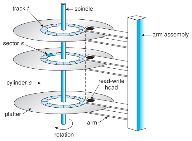
Modern DBMSs generally work with logical block addresses and database pages rather than directly calculating track and sector positions.
Important points
- Data stored on secondary storage must generally be brought into memory before the CPU can process it.
- Database systems transfer data in pages or blocks rather than fetching an arbitrary byte from disk for every operation.
- A disk access can be expensive compared with accessing data already present in RAM.
- Database performance is therefore strongly influenced by the number of page reads and writes.
How database tables are stored
Consider an Employee table with the following properties:
| Property | Value |
|---|---|
| Number of records | 100 |
| Size of each record | 128 bytes |
| Block size | 512 bytes |
Step 1: Calculate records per block
Step 2: Calculate the number of blocks
Therefore, the table requires 25 blocks, assuming each block contains four complete records and there is no additional storage overhead.
Full table scan
Suppose we want to find an employee whose ID is 75.
Without an index, the DBMS may have to examine the table's data pages one by one.
- Best case: The record is found on the first page.
- Worst case: All 25 pages are examined.
- If every page must be checked, the number of page reads is 25, assuming none is already cached.
This operation is called a full table scan.
A full table scan is not always bad. It can be efficient when the table is small or the query needs a large percentage of its rows. However, it may become expensive for large tables when only a few records are needed.
Indexing in DBMS
What is an index?
An index is an auxiliary data structure that helps a DBMS locate records without scanning every data page.
It generally stores search-key values and references that help locate the corresponding data.
- Key (e.g., Employee ID) — 10 bytes
- Record Pointer (points to the actual record on disk) — 6 bytes
Think of an index like the index at the back of a textbook. Instead of reading every page to find a topic, you use the index to jump to the relevant page.
For example
SELECT *
FROM Employee
WHERE employee_id = 75;
Without a suitable index, the database may perform a full table scan. With an appropriate index, it can search the index and then retrieve the required record or records.
How an index works
Consider this simplified index
| Employee ID | Record pointer |
|---|---|
| 10 | Page 1, record 1 |
| 25 | Page 1, record 4 |
| 50 | Page 2, record 2 |
| 75 | Page 4, record 1 |
When the DBMS searches for employee ID 75:
- It searches the index for key 75.
- It obtains the relevant record location or data-page reference.
- It accesses the corresponding data page.
- It retrieves the record.
The index is typically much smaller than the complete table, so searching it can require substantially fewer page accesses.
Numerical example: Why indexing helps
Continue with the Employee table.
Assume
- 100 records
- 25 data blocks
- 512-byte blocks
- Each simplified index entry occupies 16 bytes: 10 bytes for the key and 6 bytes for the pointer.
The pointer size and key size here are illustrative, not universal database specifications.
Index entries per block
Index blocks required
For a simple linear scan of this index, followed by one data-page access, the worst-case estimate is:
This is compared with up to 25 data-page reads for a full table scan.
Advantages of indexing
- Faster lookups using indexed columns.
- Faster filtering for suitable
WHEREconditions. - Improved performance for many joins.
- Efficient ordering and range queries with suitable indexes.
- Potentially reduced disk I/O.
Disadvantages of indexing
- Requires additional storage.
- Increases the cost of
INSERT,UPDATE, andDELETEoperations because affected indexes must be maintained. - Too many indexes can increase storage and maintenance costs.
- An index may not be useful when a query retrieves most of the table.
- Poor index selection can increase rather than reduce query cost.
Main categories of indexes
Indexes can be classified along different, partly independent dimensions.
| Classification | Types | What it describes |
|---|---|---|
| By organization | Clustered, non-clustered | How the index relates to data storage |
| By density | Dense, sparse | How many search-key entries are maintained |
| By structure | B+ Tree, hash, bitmap, etc. | How the index organizes and searches keys |
| By constraint | Unique, non-unique | Whether duplicate indexed values are permitted |
| By coverage | Covering, non-covering | Whether an index contains everything a query needs |
| By storage model | Row-oriented, column-oriented | How the underlying table data is stored |
These classifications should not be confused. For example, a unique index can also be a B+ Tree index, and a clustered index may have different implementation details in different database systems.
Dense Index and Sparse Index
These two index types are distinguished by the number and placement of index entries.
Dense index
A dense index contains an index entry for every record in the database.
Structure
Each index entry stores
- Key
- Pointer to the actual record
Employee records
| Employee ID | Record |
|---|---|
| 1 | Record 1 |
| 2 | Record 2 |
| 3 | Record 3 |
| 4 | Record 4 |
Dense index
| Key | Pointer |
|---|---|
| 1 | Record 1 |
| 2 | Record 2 |
| 3 | Record 3 |
| 4 | Record 4 |
Advantages
- Provides a direct route to the matching record or records.
- Supports fast searches.
- Does not require searching through an entire data block to locate the indexed key.
Disadvantages
- Requires more index storage.
- Increases index maintenance work during data modifications.
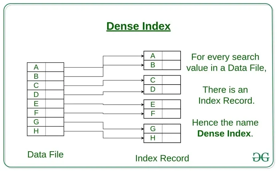
Sparse index
A sparse index contains index entries for only some records, not all.
Typically, there is one index entry per block.
Structure
Each index entry stores
- Key
- Pointer to a block (not the exact record)
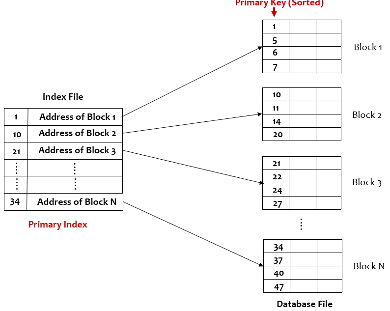
Suppose we search for employee ID 5.
- The index shows that block 2 begins with key 4.
- The DBMS identifies block 2 as the relevant block.
- It searches within that block to find key 5.
Advantages
- Requires less storage.
- Has fewer entries to maintain.
- Can be efficient when data is ordered and blocks contain many records.
Disadvantages
- May require additional searching within the selected data block.
- Generally requires an ordered data file or another suitable organization to identify the correct block reliably.
Dense index vs. sparse index
| Feature | Dense index | Sparse index |
|---|---|---|
| Entries | Every search-key value or record | Selected search-key values |
| Storage | Higher | Lower |
| Search | More direct | May require a local scan |
| Underlying data order | Depends on implementation | Typically requires ordered data |
| Maintenance | Usually more entries to update | Often fewer entries to update |
Interview point: Sparse indexing works especially well with ordered data. A classic sparse index stores one entry per data block, often pointing to the first key in that block.
Multi-Level Indexing, B Trees & B+ Trees
Multi-Level Indexing
When the table grows (e.g., 1000 rows → 40 index blocks), searching the index itself becomes slow. Solution: add an index on top of the index.
Level 1: Index entries that point to the underlying data blocks or lower-level index pages.
Level 2: Index entries that point to Level 1 pages.
Higher levels: Additional index pages that direct the search toward the appropriate lower level.
Database table: 250 blocks
Level-1 index: 40 blocks
Level-2 index: 2 blocks
Search: 2 blocks (L2) + 1 block (L1) + 1 data block = 4 blocks
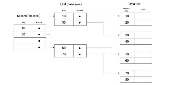
Repeatedly building indexes on lower-level indexes creates a hierarchical structure.
When rotated visually, multi-level index looks exactly like a tree — this is the origin of B Trees.
Problem: Managing these index levels manually is impractical. We need self-managing, automatically growing/shrinking multi-level indexes → This motivates balanced tree structures such as B-Trees and B+ Trees.
M-Way Search Trees
An extension of Binary Search Trees (BST) where each node can have M children and M−1 sorted keys.
| Property | Binary search tree | M-way search tree |
|---|---|---|
| Maximum children | 2 | |
| Maximum keys per node | 1 | |
| Key order | Based on left/right relationships | Keys within each node are sorted |
| Search paths | One of up to two branches | One of up to branches |
A binary search tree is the special case .
Node structure (M = 4):
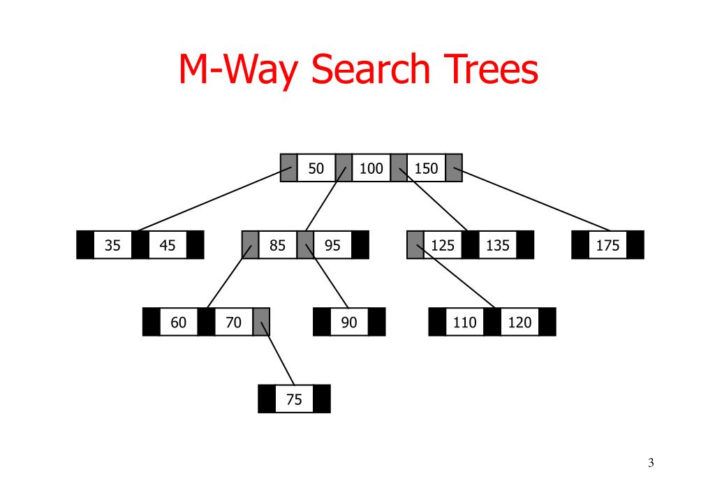
Problem with ordinary M-way search trees
An M-way search tree does not automatically remain balanced.
If insertions create a highly uneven structure, the height may become large, and searches can approach linear time in the number of keys.
The solution is to impose structural constraints. B-Trees and B+ Trees are balanced multiway search trees designed for this purpose.
B Trees
B Trees = M-Way Search Trees with rules to control structure.
A B-Tree is a self-balancing multiway search tree in which keys are maintained in sorted order, all leaves are at the same depth, and insertion or deletion operations preserve the tree's structural rules.
B-Trees are suitable for storage systems because each node can be sized to fit a disk page and contain many keys and child pointers.
Properties of a B-Tree
Using the common definition where the order is the maximum number of children:
- Each node can have at most children.
- Each node can have at most keys.
- Except for the root, each internal node has at least children.
- A non-root node therefore has at least keys.
- If the root is not a leaf, it has at least two children.
- All leaves occur at the same depth.
- Keys within each node are sorted.
- A B-Tree remains balanced as records are inserted and deleted.
- Creation is bottom-up (tree grows upward)
B-Tree node structure
A B-Tree node can contain
- Sorted keys.
- Child pointers for navigating to other nodes.
- Data pointers or record references (— one per key) associated with keys, depending on the implementation.
This means that a search can sometimes finish at an internal node rather than reaching a leaf.
Insertion and splitting
When a node is full and a new key must be inserted, the node may split. A separator key is promoted to the parent so that the search-order property is preserved.
If the root splits, a new root is created, increasing the height by one.
Example using a B-Tree of order 4, with at most three keys per node:
Insert the keys 10, 20, and 40:
10 | 20 | 40
One node has reached its maximum capacity.
Now insert 50. Under the convention that splitting a full node promotes a middle separator, the tree reorganizes so the keys remain ordered and each node respects its capacity. The exact split arrangement depends on the insertion algorithm and overflow convention.
For an overflow of four keys, one possible resulting arrangement is:
Illustrative split for an overflow of four keys; splitting rules vary by convention.
Advantages of B-Trees
- Balanced height.
- Efficient exact-key search.
- Efficient insertions and deletions.
- Suitable for disk-based storage because nodes can hold multiple keys.
- Avoids the deep structure that can occur in an ordinary unbalanced search tree.
Key Differences from B Trees
| Feature | B Tree | B+ Tree |
|---|---|---|
| Record pointers | Every node (all keys) | Leaf nodes only |
| Keys in leaves | Some keys may only be in internal nodes | All keys must appear in leaf nodes |
| Leaf connectivity | Not connected | Linked list (left to right) |
| Index type | Mix | Internal = sparse index, Leaves = dense index |
Limitations for database indexing
B-Trees can store records or record pointers in internal nodes as well as leaves. As a result, their leaf nodes do not necessarily contain every search key.
This is not inherently incorrect, but it is less convenient for ordered range scans when compared with a design that stores all entries at the leaf level and links the leaves together.
This leads to the B+ Tree.
B+ Trees
B+ Trees are a modification of B Trees better suited for database indexing.
How B+ Trees Work
- Internal (non-leaf) nodes store only keys for routing — no record pointers
- Leaf nodes store all keys + record pointers
- Any key that appears internally is duplicated at the leaf level
- All leaves are at the same level and linked together like a linked list
Why B+ Trees Are Better for Databases
Find by ID: Traverse from root → internal nodes → leaf. Always exactly log(n) disk reads (predictable).
Searching in a B+ Tree
Suppose we need to find employee ID 45.
- Start at the root.
- Compare 45 with the separator keys.
- Follow the appropriate child pointer.
- Repeat until reaching the leaf page.
- Find key 45 in the leaf.
- Use its record reference to retrieve the actual row if the leaf does not already contain the row.
The number of page accesses is related to the height of the tree, not the total number of rows scanned sequentially.
Range query (e.g., rows 100–600):
- Reach the starting leaf via tree traversal
- Then linearly scan the linked leaf nodes without going back to the root
- Extremely efficient — leaves are already sorted and connected
Suppose we execute
SELECT *
FROM Employee
WHERE employee_id BETWEEN 100 AND 600;
A B+ Tree can process the query efficiently:
- Search for the first relevant key, 100.
- Locate its leaf page.
- Scan entries in sorted order.
- Follow the leaf-level sibling pointers into subsequent pages.
- Stop when keys exceed 600.
The typical index traversal cost can be expressed as:
Here, is the number of indexed entries and is the number of matching entries examined, abstracting away page sizes and output costs.
Insert/Update/Delete
- Read only the relevant B+ tree nodes (a few disk blocks)
- Modify in memory, flush back to disk
- No need to rewrite the entire file
- Changes are local — other blocks untouched
Why Databases Use B+ Trees (Not B Trees)
B Trees store data in internal nodes too, which means range queries require jumping around the tree. B+ Trees force all data to the leaf level, enabling:
- Predictable read time for any row
- Efficient sequential scan for range queries via the leaf linked list
Both SQL (MySQL, PostgreSQL) and NoSQL (MongoDB's WiredTiger engine) use B+ Trees to store table/collection data on disk.
Summary Diagram
Index Types: Clustered & Non-Clustered
Clustered and Non-Clustered Indexes
This classification describes the relationship between the index and the organization of the underlying table.
Clustered index
A clustered index organizes the table's data according to the clustered search key.
When you create a clustered index on a column (e.g., CustomerID), two things happen:
- The database physically reorders all the data pages so rows are sorted by that column — lowest to highest.
- It builds a B-tree (Balanced Tree) — an upside-down hierarchical structure:
- Root node — one index page at the top
- Intermediate nodes — index pages pointing to other index pages
- Leaf nodes — the actual data pages (physically sorted)
To find a row, the database traverses from root → intermediate → leaf, following pointers. For a 20-row table split across 4 pages, finding row 14 takes just 3 hops (root → intermediate → data page), reading only 1 data page instead of all 4.
Key rules
- You can only have one clustered index per table — because data can only be physically sorted one way
- Best column: one that is unique and rarely updated — the primary key is ideal (unique + never changes)
- Also great for range queries (e.g.,
WHEREidBETWEEN10AND50)
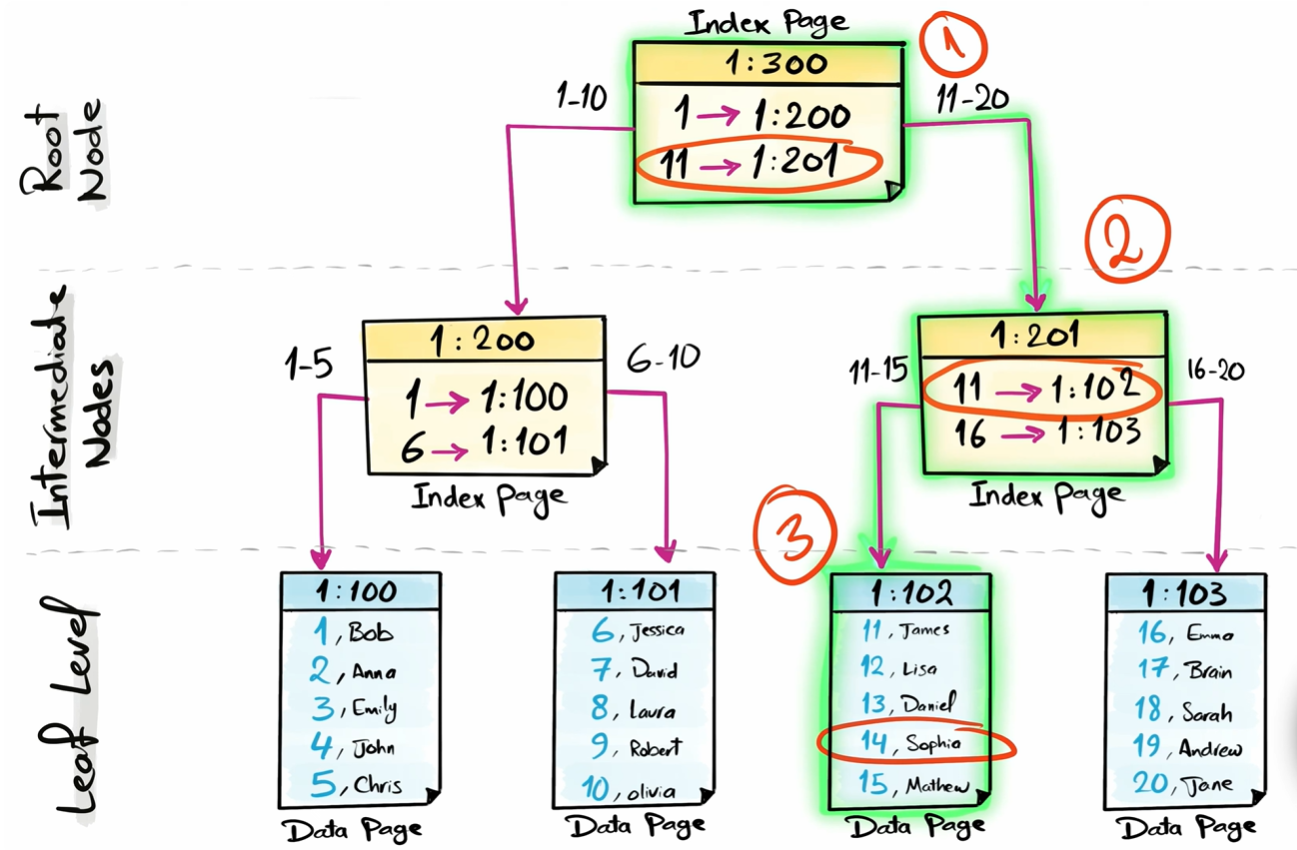
Non-clustered index
A non-clustered index is a separate index structure whose leaf entries contain the indexed key and a locator for the corresponding row or clustered key.
A non-clustered index does not touch or reorder the actual data. Instead, it builds a completely separate B-tree structure:
- Root and intermediate nodes — same as clustered index (index pages pointing to index pages)
- Leaf nodes — index pages containing row locators (row identifiers, or RIDs), each storing the exact file ID + page number + row offset where the actual row lives in the data pages
The data pages themselves remain in their original heap order and are not part of this B-tree at all.
To find a row, the traversal goes: root → intermediate → leaf (row locator page) → jump to exact row in data page. This is one extra hop compared to a clustered index, making it slightly slower for reads.
Key rules
- You can create as many as needed — each is a separate B-tree with pointers to the same data
- Best for columns used in
WHEREclauses,JOINconditions, or exact-match lookups on non-primary-key columns - Writes are faster than with a clustered index, since the physical data pages don't need re-sorting
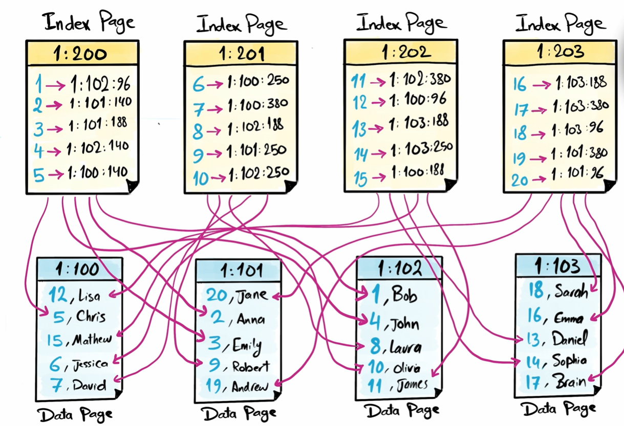
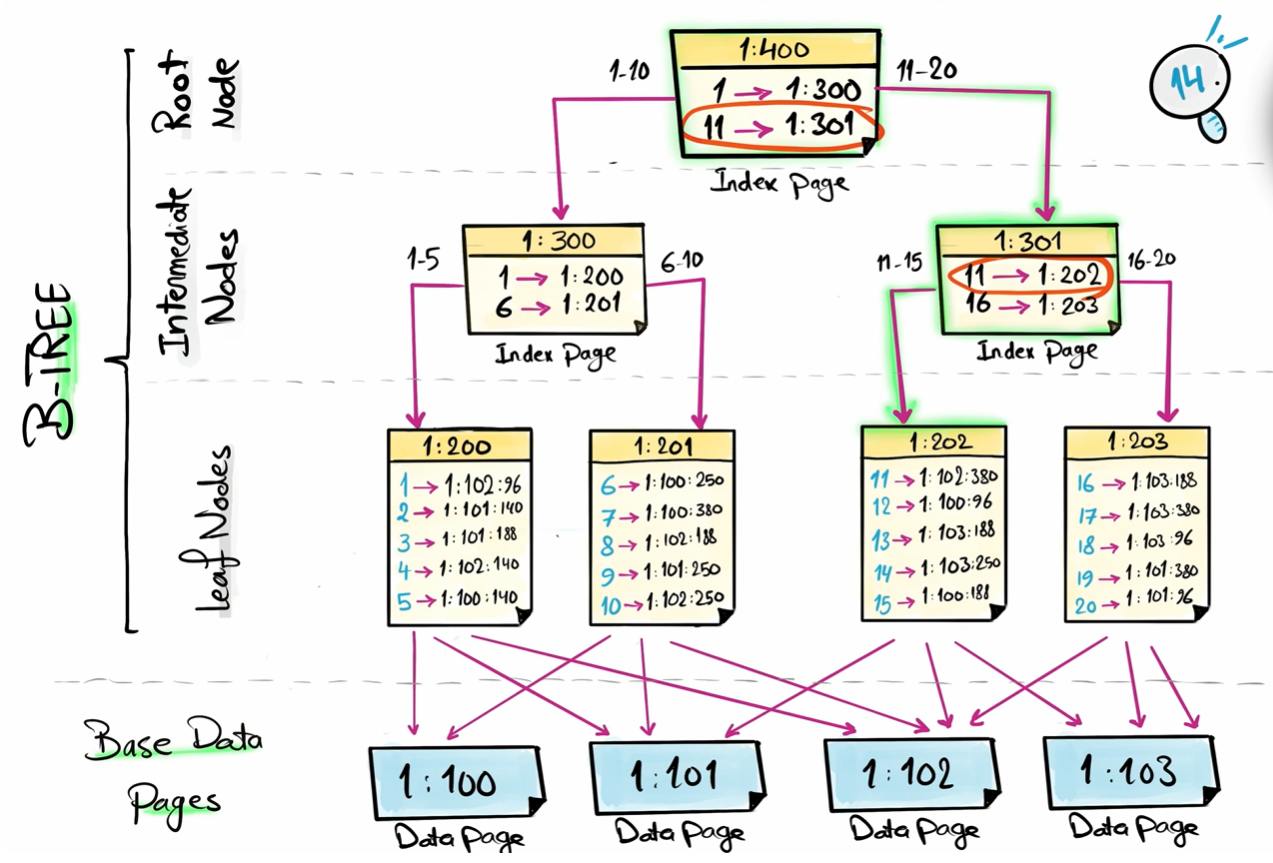
Tradeoffs at a glance
| Clustered | Non-clustered | |
|---|---|---|
| Max per table | 1 | Unlimited |
| Leaf level contains | Actual data pages | Row locator pointers |
| Read speed | Faster | Slightly slower (extra hop) |
| Write speed | Slower (must re-sort) | Faster |
| Storage | More efficient | Uses extra space for index pages |
| Physical data order | Changed | Untouched |
Database Replication
What is database replication?
Database replication is the process of copying and maintaining the same data across multiple servers so that the system continues to work even if one server goes down.
The result is several live copies of your database running simultaneously.
The main objectives are
- High availability.
- Improved read performance.
- Fault tolerance.
- Disaster recovery.
- Reduced latency for users in different geographic regions.
A classic example: an e-commerce site uses one primary database to handle orders (writes), and a fleet of read replicas to serve product listings, search results, and user profiles (reads).
Replication creates multiple copies of data. It does not, by itself, divide the dataset into smaller pieces.
How it works
- A primary database is designated as the single source of truth for all changes.
- Replica databases are configured to receive data from the primary.
- Every insert, update, or delete on the primary is recorded — typically in a transaction log or via change data capture (CDC).
- Those captured changes are transmitted to replicas over the network, either instantly or at intervals.
- Replicas apply the changes to bring themselves in sync.
- The system continuously monitors sync state and handles delays or conflicts.
- Applications read from replicas and write to the primary (or in some models, write to any node).
Types of replication
1. Master-slave (primary-replica)
One master handles all writes. Slaves receive a copy and serve reads.
- Write path: master only
- Read path: any slave
- Failure: if the master dies, a slave must be manually or automatically promoted
- Best for: read-heavy applications — social feeds, product catalogues, CMS
The key limitation is that write capacity doesn't scale — everything still flows through one master. Also introduces replication lag, meaning slaves may be slightly behind the master.
2. Master-master (multi-master)
Two or more nodes each accept reads and writes. Changes on one are synced to the others.
- All nodes are peers — any can accept a write
- Requires conflict resolution: if two nodes update the same row simultaneously, the system must decide which wins (last-write-wins, vector clocks, application logic, etc.)
- Best for: multi-datacenter setups, collaborative platforms, globally distributed writes
More powerful but significantly more complex to manage. A misconfigured conflict resolution strategy can silently corrupt data.
3. Snapshot replication
A full copy of the entire database is taken at a point in time and sent to subscribers.
- Not real-time — the snapshot represents the state at one moment
- Simple to set up and restore from
- Best for: data warehousing, analytics, compliance/auditing, periodic reporting
- Not suitable where data changes constantly and freshness matters
4. Transactional replication
Every individual transaction (insert/update/delete) is captured and sent to subscribers in near real-time, one change at a time.
- Maintains high consistency across locations
- Publisher → distributor → subscriber pipeline
- Best for: financial systems, live dashboards, online gaming, any scenario requiring fresh data everywhere
Adds some overhead on the publisher and requires careful agent/distributor configuration.
5. Merge replication
Both the publisher and subscribers can modify data independently. Changes are merged during synchronisation, with conflicts detected and resolved.
- Two-way (bidirectional) sync
- Works for intermittently connected systems — devices can work offline and sync later
- Best for: field service apps, healthcare devices, mobile apps that work without connectivity
Conflict resolution here is the hardest problem — the same record might be edited on two devices with no connectivity between them.
Replication configurations (how it's timed)
Synchronous replication
The primary waits for at least one replica to confirm receipt before committing the transaction. This guarantees no data is lost if the primary crashes immediately after a write.
- Strong consistency
- Higher latency — every write is slower because it waits
- Used when data loss is completely unacceptable (banking, payments)
Asynchronous replication
The primary commits immediately and sends changes to replicas in the background. Replicas catch up with a slight delay.
- Low latency — primary doesn't wait
- Risk of data loss: if the primary crashes before a replica receives the change, that change is gone
- Acceptable in most read-heavy web apps where slight lag is tolerable
Semi-synchronous replication
A middle ground: the primary waits for confirmation from at least one replica, then proceeds. Other replicas catch up asynchronously.
- Balances consistency and performance
- Ensures at least one copy always has the latest data
Why replication matters in system design
High availability — if the primary goes down, a replica can be promoted to take over. The system keeps running with minimal or zero downtime.
Load balancing — a load balancer can route all read queries to replicas, leaving the primary free to handle writes. This is one of the most common and impactful performance optimisations.
Disaster recovery — geographically separated replicas survive regional outages, data centre fires, or infrastructure failures.
Fault tolerance — individual server failures don't take the system down because traffic shifts to surviving replicas automatically.
Data locality — replicas placed physically close to users in different regions reduce latency for those users significantly.
Scalability — adding more read replicas lets the system handle more concurrent users without touching the primary.
Challenges
Replication lag — in async replication, replicas can be seconds (or more) behind the primary. A user who just wrote data may immediately read a replica and see stale data — a common source of bugs in distributed systems.
Conflict resolution — in multi-master setups, simultaneous writes to the same row on different nodes create conflicts. No universal correct answer — strategy depends on the domain (last-write-wins, application-level logic, manual resolution).
Complexity — setting up and maintaining replication pipelines, monitoring lag, handling failovers, and configuring agents/distributors requires significant expertise.
Write bottleneck — master-slave does nothing for write scalability. If the app is write-heavy, replication alone doesn't help — you need sharding or master-master.
Consistency vs. latency tradeoff — synchronous gives you consistency but costs latency. Async gives you speed but risks lost writes. You cannot fully have both.
Cost — every replica is another server. Large-scale deployments with many replicas across multiple regions are expensive to run and maintain.
Data Partitioning
Data Partitioning
Data partitioning divides a large table or dataset into smaller logical parts called partitions.
Partitioning may occur within one database server or across multiple servers.
The objectives include
- Better query performance.
- Partition pruning.
- Easier maintenance.
- Improved manageability of large tables.
- Parallel processing in suitable systems.
There are two main types
- Horizontal Partitioning → splits data by rows (e.g., users by region)
- Vertical Partitioning → splits data by columns (e.g., separating personal info from transaction data)
The six partitioning methods
1. Horizontal partitioning
Horizontal Partitioning divides data by rows, but all partitions may still exist on the same server. When these horizontal partitions are placed across multiple servers, the approach is called Sharding.
Each partition contains the same logical columns but a different subset of rows.
Example
Original table
| User ID | Name | Region |
|---|---|---|
| 1 | Asha | India |
| 2 | Ravi | US |
| 3 | Neha | India |
| 4 | Omar | Europe |
Possible horizontal partitions
- Partition 1: users in India.
- Partition 2: users in the US.
- Partition 3: users in Europe.
All partitions share the same logical schema.
Advantages
Horizontal partitioning divides a table into multiple parts by distributing rows across different partitions or servers.
• Scalability: Allows parallel processing of large datasets across multiple nodes.
• Load Balancing: Distributes workload evenly, reducing system bottlenecks.
• Fault Tolerance: Each partition works independently, improving reliability during failures.
Disadvantages
Despite its scalability benefits, it introduces some complexity in database operations.
• Complex Joins: Joins across multiple partitions can be slower and harder to manage.
• Data Skew: Uneven data distribution may cause certain partitions to handle more load than others.
Vertical Partitioning
Vertical partitioning divides a table by columns. Each resulting structure contains a subset of the original columns, with a shared identifier or key used to associate related rows.
Example
Original Users table
Users(
    user_id,
    name,
    email,
    bio,
    avatar,
    preferences
)
Vertical split
Users_Core(
    user_id,
    name,
    email
)
Users_Profile(
    user_id,
    bio,
    avatar,
    preferences
)
The shared user_id connects the two structures.
Good for: tables with many columns where only a subset is frequently accessed; reduces I/O by not reading unused columns
Advantages
Vertical partitioning divides a table by separating columns into different partitions based on usage or functionality.
- Better Query Performance: Reduces data read by isolating frequently accessed columns.
- Efficient Retrieval: Fetches only needed columns, saving I/O and storage.
- Easier Schema Changes: Simplifies adding or removing columns.
Disadvantages
Although useful for column-level optimization, it can introduce additional query complexity.
- Query Complexity: Queries may need to access multiple partitions.
- Slower Joins: Combining data from different partitions adds overhead.
- Limited Scalability: Not ideal for datasets with rapidly growing columns.
3. Key-based Partitioning
Divides data based on a specific key or attribute, with each partition holding all data related to that key. Common in distributed systems for uniform data distribution and efficient key-based lookups.
A hash function on the key determines the destination partition.
Good for: point lookups — "give me all data for user X" is fast because it's all in one partition
Disadvantages
Watch out for: hot keys cause one partition to handle disproportionate load; range queries are inefficient since consecutive keys may scatter across partitions.
4. Range partitioning
Partitions are defined by value ranges — date ranges, ID ranges, alphabetical ranges. A query for data within a range hits only the relevant partition(s).
- Good for: time-series data, logs, any naturally ordered data; range queries are highly efficient
- Watch out for: if recent data is queried far more than old data (which is typical), the "current" partition is always hot; requires ongoing maintenance as ranges fill up
5. Hash-based partitioning
A hash function is applied to the data and the output determines which partition it goes to. Similar to key-based but the hash randomises placement rather than grouping by key identity.
- Good for: even distribution across partitions; write-heavy workloads where you want to spread load uniformly
- Watch out for: terrible for range queries (consecutive values are randomised across partitions); resharding requires rehashing all data
6. Round-robin partitioning
Records are assigned to partitions in a rotating sequence — record 1 to partition 1, record 2 to partition 2, record 3 to partition 3, record 4 back to partition 1, and so on.
- Good for: achieving near-perfect write distribution without needing a meaningful key; simple to implement
- Watch out for: no data locality — related records are spread everywhere; any query that needs to find "all records matching X" must scan all partitions; poor fit for analytical or key-based queries
Partition pruning
Partition pruning occurs when the DBMS determines that some partitions cannot contain rows matching a query and skips them.
Example
SELECT *
FROM Orders
WHERE order_date >= '2026-01-01'
  AND order_date <  '2026-02-01';
If the table is partitioned by month, the DBMS may scan only the January 2026 partition.
Pruning depends on the partition definition, the query predicates, and the database optimizer.
Database Sharding
What is sharding?
Database sharding is a horizontal scaling technique where a large dataset is split into smaller chunks called shards, each stored on a multiple database instances.
Every shard holds the same schema as the original database, but each row appears in exactly one shard — there is no duplication of data across shards (unlike replication, which copies everything).
The key idea: instead of one massive database server struggling under load, you spread the data across many smaller servers, each handling only a fraction of the total dataset.
Sharding key
A shard key is the attribute or combination of attributes used to determine where a record is stored.
Examples
user_idcustomer_idorder_date- (region,
customer_id)
A good shard key should distribute data and workload reasonably evenly while supporting common query patterns.
A poor shard key may cause:
- Uneven storage distribution.
- Hot partitions.
- Expensive cross-shard queries.
- Difficult rebalancing.
Sharding methods
1. Key-based (hash-based) sharding
A hash function is applied to a shard key (e.g., customer_id) to determine which shard stores that row. For example, with 3 shards: shard = customer_id % 3. The remainder (0, 1, or 2) decides the destination.
- Pros: uniform distribution if the key is well-chosen; consistent placement means you always know where a record lives without a lookup
- Cons: adding or removing shards requires rehashing everything; hot keys cause uneven load; choosing a bad shard key breaks the uniformity
2. Range-based sharding
Data is divided by value ranges of a column. For example, customers whose names start with A–P go to shard 1, Q–Z to shard 2. Or orders from January–June go to shard 1, July–December to shard 2.
- Pros: natural fit for time-series or ordered data; range queries are efficient since all matching data is in one shard
- Cons: uneven distribution if data is skewed toward certain ranges (e.g., most customers have names starting with S); one shard can become a hotspot
3. Directory-based sharding
A central lookup service (a directory or lookup table) maps each shard key to its shard location. Every query first asks the directory which shard to go to, then routes there.
- Pros: flexible — you can move data between shards without changing application logic; supports dynamic scaling
- Cons: the directory is a single point of failure; every query incurs an extra network hop to the directory, increasing latency
Sharding vs. partitioning — the distinction
These terms are often used interchangeably, but there is a meaningful difference. Partitioning is the general concept of dividing data — it can happen on a single machine. Sharding is a specific type of horizontal partitioning where each partition lives on a completely separate database server, giving you true distributed scale. All sharding is partitioning, but not all partitioning is sharding.